Preprocessing Datasets
-
Intro
-
Finding and Selecting a Dataset
-
Loading the Data Set
-
Feature Selection
-
Cleaning the Dataset
-
Analysing Dataset Distribution
-
Conclusion
-
Useful Links
Information
| Primary software used | Jupyter Notebook |
| Course | Preprocessing Datasets |
| Primary subject | AI & ML |
| Secondary subject | Machine Learning |
| Level | Intermediate |
| Last updated | November 12, 2025 |
| Keywords |
Responsible
| Teachers | |
| Faculty |
Preprocessing Datasets 0/7
Preprocessing Datasets
Explanation on how to preprocess a dataset for research purpuses with Python coding in Google Colab.
In this tutorial, you will learn how to clean the dataset, a crucial step in machine learning sometimes referred to as pre-processing the data. The goal is to prepare the dataset for quantitative research or machine learning tasks. You can follow the tutorial ‘Getting Started with Python in Google Colab’ to get familiar with Python coding and importing a dataset in your Jupyter Notebook. If you want to know more about the theory of using big data, where to find datasets and the importance of data cleaning you can go to the first chapter of the workshop ‘Pre-processing data for ML purposes’.

Exercise file To discuss and understand data set cleaning, we will use the WoON21 dataset. The dataset consists of data on the composition of households, the housing situation, housing preferences, housing costs and moving behaviour. The survey is conducted every three years by the Dutch government and is an important basis for the housing policy in The Netherlands. You can download the dataset on the BK3WV4 Brightspace page. If you want to know more about the WoON dataset you can visit the dashboard of Woononderzoek Nederland. You can also download your own selection of the dataset at the Citavista Databank in case you do not have access to the Brightspace. Additionally, here you can download additional information, such as the explanation of the variables in the WoON2021 dataset in both Dutch and English.
Preprocessing Datasets 1/7
Finding and Selecting a Datasetlink copied
In this tutorial, we will introduce a research question that we could answer using the dataset. The dataset provides a lot of data, and the goal is to find and analyse the correct information within the data that might be relevant to answering the research question.
What we will be looking for in the data are information that can predict how satisfied people are with their homes. What data is useful to make such prediction? We will select the information from the dataset that relate to the research question. To make our prediction for how satisfied people are with their neighbourhood in the Netherlands, we will use a common machine learning algorithm for classification. Maybe our hypothesis is that the closer the local urban amenities are the higher neighborhood satisfaction is.
For the purposes of this tutorial, we will ask the question:
How does the accessibility of local urban amenities impact the neighbourhood satisfaction of Dutch households?
Note that the dataset must fit within the boundaries of the research. If the research question concerns Western countries, a dataset containing information from Asian countries could be a mismatch. Or if the dataset has information on urban areas but the research question focuses on rural areas, this could also be a mismatch.
Preprocessing Datasets 2/7
Loading the Data Setlink copied
Let’s run through the basics of how to load your dataset. This chapter shows two ways of how to import a CSV dataset. The first sub-chapter shows how you can import the dataset from a local storage. The second sub-chapter shows how you can import the dataset from a google drive. You can follow one of the two steps. The last sub-chapter is a short explanation on how to inspect the dataset.
In the case of the WoON dataset, the raw download consists of a .csv file. We will load the data set from a . csv file into a Pandas DataFrame.
IMPORTANT: after you download the CSV file from the previous page, it will be in a ZIP folder. You need to unzip the folder by right clicking and selecting “extract all”. This will create a new regular folder in the same location. Navigate to this folder and use the CSV file that’s in it to upload into your Google Drive or load via a file path.
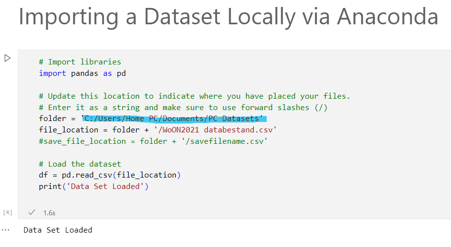
Importing a Dataset Locally via Anaconda
First, import the needed library to read CSV files; in this case, import Pandas as pd. Next, load the entire . csv file using the code in the provided Jupyter Notebook. Do not forget to change the folder location highlighted in blue below. Lastly, load the dataset as a DataFrame. You can find the full code below.
# Import libraries
import pandas as pd

# Update this location to indicate where you have placed your files.
# Enter it as a string and make sure to use forward slashes (/)
folder = ''
file_location = folder + '/FeatureSelection_WoON21_dataset.csv'
#save_file_location = folder + '/savefilename.csv'

# Load the dataset
df = pd.read_csv(file_location)
print('Data Set Loaded')
Importing a dataset with Google Colab
If you are following along in Google Colab and you want to connect the CSV file from the Google Drive, the steps are as follows:
- Import the needed libraries of Google Colab and Pandas.
- Define the file path and load the CSV file in a Dataframe.
- Make sure to mount the drive once and find the file path, as shown in the previous tutorial’s importing datasets section.
Below shows the code to load the dataset from Google Drive, load it to a DataFrame and view the dataset.
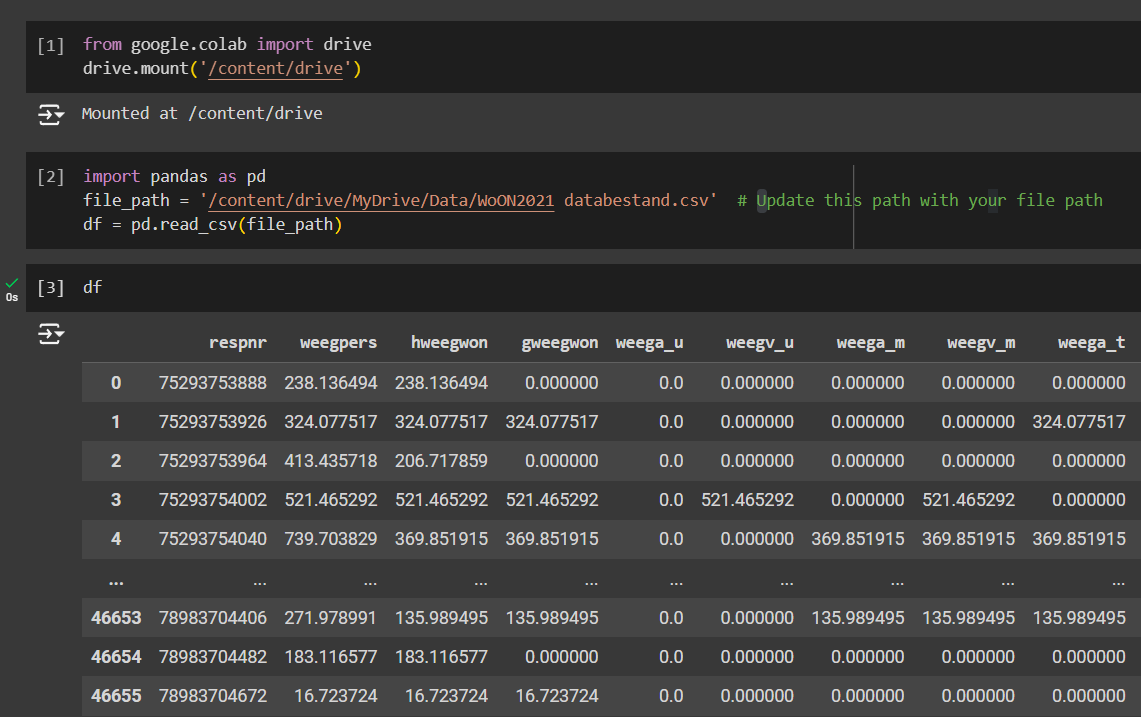
from google.colab import drive
drive.mount('/content/drive')

import pandas as pd
file_path = ''
df = pd.read_csv(file_path)
Inspecting the Imported Dataset
Now that you have loaded the datasets, let’s inspect the information provided to see which is relevant to us.
Notice that if you are attempting to view the columns using Pandas function df.columns, it’s likely that it won’t display all of them due to the size of the dataset. One workaround way to view all the columns in the output is to turn it into a list using this code: print(list(df.columns)).
In the output field, you can view all the column information in there. An alternative method is to view the entire table by making Pandas display all the columns. To do this, you will need to change the default setting like this: pd.set_option(‘display.max_columns’, None).
And to turn it back to default, reset it using this code:
pd.reset_option('display.max_columns')
Do you find interesting information for your research question? In this step you can view all the features that may be relevant to your research question so that we can begin our dataset cleaning step and prepare the data for machine learning.
Preprocessing Datasets 3/7
Feature Selectionlink copied
Features is a common terminology in machine learning. A feature is a data that can be used as input to predict an outcome. For example, the spatial features in the neighbourhood that predict satisfaction. Features are anything that we can describe and measure numerically, such as the distance between household to amenities. This includes abstract or subjective concepts like satisfaction can be given a scale, i.e. a 5-point scale. This section will show you how to select the features from the dataset that contributes to neighbourhood satisfaction.
Checking Null Values of All Columns
We can use Matplotlib to visualize the null values in all the features. Import matplotlib to visually graph the null values:

import matplotlib.pyplot as pltLet’s first check the overall dataset for missing values. We can use Pandas to help with this using the function df.isnull().sum().
- Let’s sum up all the null values into a new variable called null_counts
null_counts = df.isnull().sum()- Then we will plot a bar chart for every feature to count the number of missing values in each feature. We set the size of the chart and create a plt.bar chart where the x-axis will be the number of features we have and y-axis will be the number of null values:
plt.figure(figsize=(12, 6)) # set the graph size
plt.bar(range(1, len(null_counts) + 1), null_counts.values)- Label the plot using the following:
plt.title('Null Values in Each Column')
plt.xlabel('Columns')
plt.ylabel('Number of Null Values')
plt.show()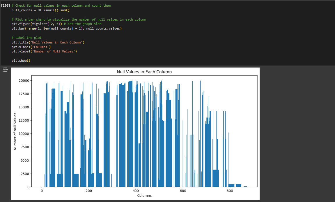
Defining the Features
Now that we have loaded the dataset inside the Jupyter Notebook, let’s make selection for the features that are relevant to our research question. Because our research question concerns the proximity of households to urban amenities, we will identify all the features that describe distances.
Upon closer inspection to the dataset, there are two keywords that describe the distances: number of amenities nearby and distance to amenities. To write a code that selects all the features using keywords that matches with our selection, you can follow this step below:
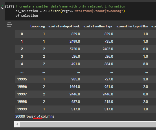
- We will use a Pandas function to filter the dataset to match with our defined keywords. The function is .filter() and in between the parentheses we add our keywords.
- The | symbol denotes an OR condition which is to find columns that have the keywords ‘vzafstand’ OR ‘vzaant’ in them.
df_selection = df.filter(regex='vzafstand|vzaant|twoonomg')- · Note that we included the satisfaction rating in the filtering step ‘twoonomg’.
An alternative method to selecting features is to name the columns you are interested in directly in a list. Below you can execute this code which will give you the exact same results but with more control over the features you want to include.
# Alternative way to select features manually:
df_selection = df[
    [
        'twoonomg',
        'vzafstandapotheek',
        'vzafstandhartspr',
        'vzafstandhartspost',
        'vzafstandziekhinclbp',
        'vzafstandziekhexclbp',
        'vzafstandbrandweerk',
        'vzafstandovdaglev',
        'vzafstandgrsuperm',
        'vzafstandbasisond',
        'vzafstandkdv',
        'vzafstandhotel',
        'vzafstandrestau',
        'vzafstandcafe',
        'vzafstandoverstapst',
        'vzafstandoprith',
        'vzafstandtreinst',
        'vzafstandbiblio',
        'vzafstandmuseum',
        'vzafstandbioscoop'
    ]
]
Data Types and Null Values
Let’s take a closer look at our features. What type of data is it? Are there any missing or NaN values? These things are helpful to know as we move forward with cleaning our data.
To let’s create a new variable called df_selection_info where it will contain information such as the number of null values and the data types. But before we execute this code, we need to capture the null count in its own variable as well as the data types.
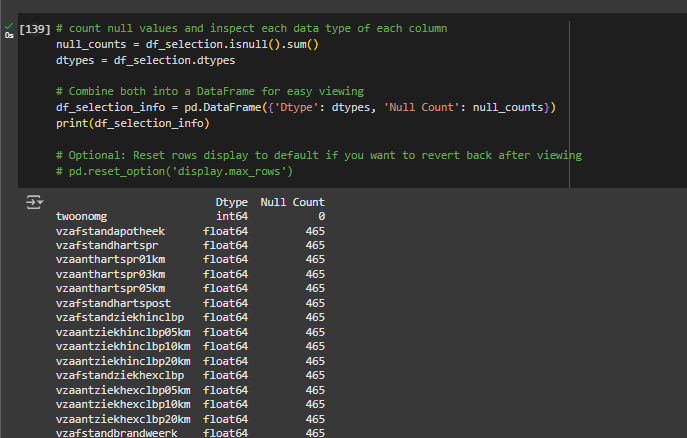
- Create two new variables, null_counts and dtypes. The variable name for our feature set is ‘x’, therefore we execute the functions as follows:
df_selection.isnull().sum
df_selection.dtypes- Next, create the df_selection _info variable and create a new DataFrame to view the results
- The pd.DataFrame() creates a new DataFrame to view the results of the variables. The proper syntax for this is
Below is the full code to view the null values and data types for any given feature set.
null_counts = df_selection.isnull().sum()
dtypes = df_selection.dtypes

# Combine both into a DataFrame for easy viewing
df_selection_info = pd.DataFrame({'Dtype': dtypes, 'Null Count': null_counts})

# Set the option to display all rows
pd.set_option('display.max_rows', None)

# Print results
print(df_selection_info)

# Optional: Reset rows display to default if you want to revert back after viewing
# pd.reset_option('display.max_rows')
We can see that the null values in all of those features. We will need to address those missing values in a subsequent step. Removing data points with null values, although will decrease the size of our dataset, is more preferred when analysing the data.
By performing the function df_selection.shape, we see that we have selected 54 features and 20000 rows.
To visually graph the null values in our entire feature set, we can use Matplotlib for plotting a graph:
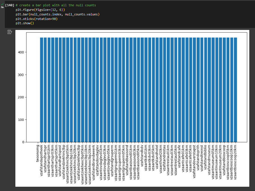
- Adjust the figure size to improve legibility of your plot by using the function plt.figure. Adjust the size arguments as needed.
- Using the same variable, null_counts plot a bar chart using Matplotlib plt.bar function.
- To make the text legible, rotate them by 90 degrees using the following function: plt.xticks(rotation=90).
- Show the plot: plt.show().
Depending on your feature set size, you may be able to see the different variation of null values. In this feature set, all the values line up to our previous findings which is 465 null values in all the features.
Your final code should look something like this:
# create a bar plot with all the null counts
plt.figure(figsize=(12, 6))
plt.bar(null_counts.index, null_counts.values)
plt.xticks(rotation=90)
plt.show()
We now move on to selecting the feature we are interested in predicting neighbourhood satisfaction, we call this the target variable.
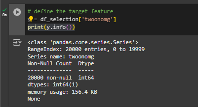
To do this, you will store the column information into a Pandas series. Let’s call this variable target.
y = df_selection['twoonomg']
print(y.info())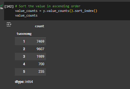
Let’s get an idea of how satisfaction is described in this dataset. Using the Pandas value_counts() function, we can view the values in this variable. For legibility, we will sort_index the list in ascending order.
value_counts = y.value_counts().sort_index()
value_counts
As you can see in the output, there are 5 possible outcomes for satisfaction that ranges from 1 to 5. Based on the documentation file for the dataset, we can see that 1 represents highest satisfaction and 5 is the lowest satisfaction.
Plotting Distribution of the Target Variable
Let’s prepare a bar chart to see the distribution of satisfaction responses. Note we use the value_counts variable as it contains the information we need to plot the graph:
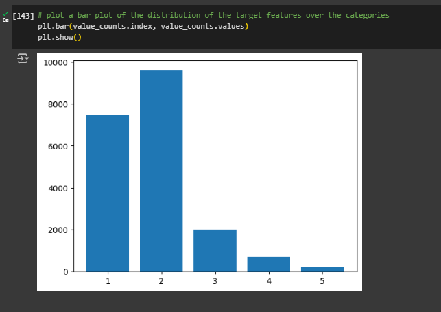
plt.bar(value_counts.index, value_counts.values)
plt.show()
We see that the majority of the responses fall between 1 and 2. There are very little data points for category 4 and 5, this could indicate outliers.
Now that you have defined both the features set and the target variable, next step is to clean the dataset, also known as the pre-processing step in machine learning.
Preprocessing Datasets 4/7
Cleaning the Datasetlink copied
Cleaning the dataset for machine learning involves several steps. In general, most data has to be pre-processed to make sure that there are no invalid values, missing values, or errors. Sometimes it is also helpful to have evenly distributed data and to avoid skewed data by removing extreme values. In summary, cleaning the dataset is an integral part of machine learning. Here in this section, we will practice a few common techniques to clean your dataset.
Removing Empty Values
Let’s start by removing empty values. As mentioned in the previous section, we need to remove NaN/null values.
First, let’s try removing all rows that contain NaN values for any column using df.dropna(). In the earlier section, we found the number of null values and we should expect our dataset to decrease by that amount.
We will begin by re-assigning our variables DataFrame and executing the df.dropna()function. To verify that the nulls were removed, execute the following print function:
# drop rows with empty values in the selected features
df_selection_removed = df_selection.dropna()

# print the results of cleaning the dataset
print('origional number of rows =',df_selection.shape[0])
print('number of rows clean dataset =',df_selection_removed.shape[0])
print('number of rows removed =', df_selection.shape[0] - df_selection_removed.shape[0])
Note: notice that the number of removed rows matches the number of null values identified in the previous section. This helps verify that the step was done correctly.
Manual Removal of Data
Let’s say that you want to narrow down your research question to see how satisfied people are of their neighbourhood in relation to non-commercial local amenities, such as schools, daycares, transit hubs, highway, hospital, etc. Let’s practice removing data from our feature set by targeting the commercial activities such as restaurants and cafes to exclude from the features set.
The first step is to define a new list variable for columns to remove, let’s call it columns_to_remove, and manually enter the names of the columns we want removed from the feature set. If you want to get a reminder for the content of the columns, you can run the function .columns.
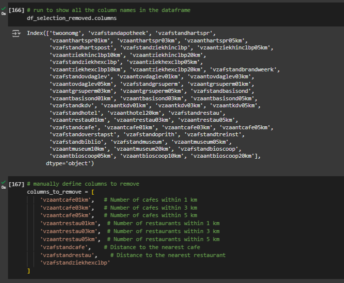
columns_to_remove = [
    'vzafstandhartspost',
    'vzafstandziekhexclbp',
    'vzafstandbrandweerk',
    'vzafstandoverstapst',
    'vzafstandoprith',
    'vzafstandcafe',
    'vzafstandrestau',
    'vzafstandziekhexclbp'
]
Now that we have defined the list of columns to be removed, we need to assign a new variable to our feature set and drop the columns that match the names from the list of columns to remove:
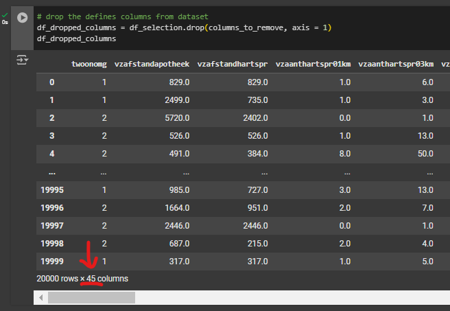
- • Create a new variable, call it df_dropped_columns, then apply the function .drop(columns_to_remove, axis = 1) on the df_selection.
- The axis argument specifies whether to remove rows, 0, or columns, 1. And because we want to remove entire columns, we specify the axis = 1.
- Print the new DataFrame and make sure the columns are removed accordingly.
You can find the full code here:
# drop the defines columns from dataset
df_dropped_columns = df_selection.drop(columns_to_remove, axis = 1)
df_dropped_columns
Now that we have our desired feature set, we want to analyse our feature set to make sure they are consistent and catch any anomalies in the data that could introduce noise in the dataset.
Preprocessing Datasets 5/7
Analysing Dataset Distributionlink copied
In this section, we will plot the data distribution of our features. This step is critical to identify extreme outliers in the data which can skew our dataset. This step is important when considering features that may have obvious errors that don’t fall in the range of the data.
We will first filter the feature selection using the .filter function and selecting features that contain the keywords ‘vzafst’. We want to inspect the outliers in this selection of features that describe distance from household to local amenities in meters.
distance_features = df_selection_removed.filter(regex='vzafst').columns
df_distance = df_selection_removed[distance_features]
df_distance.describe()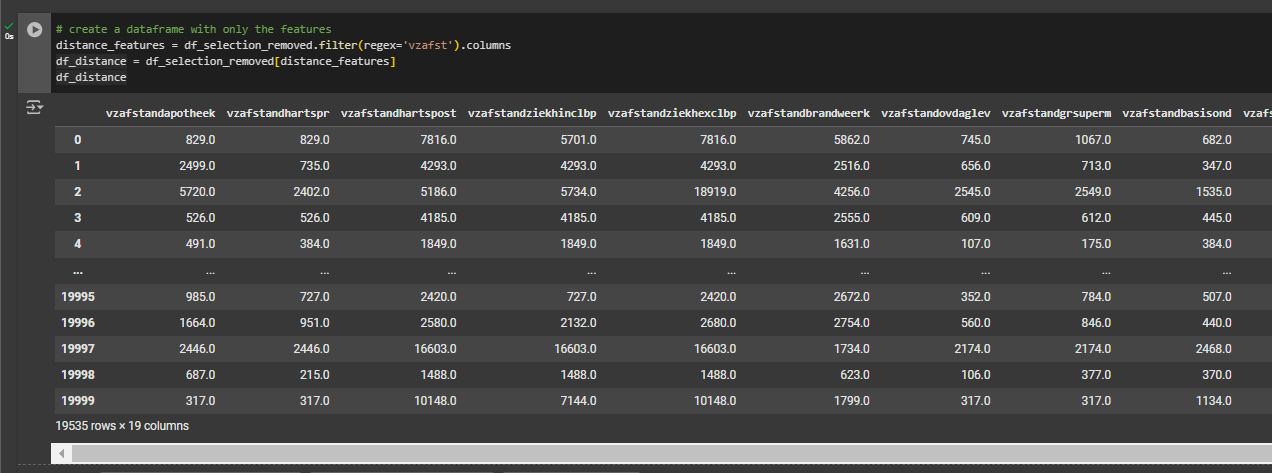

When printing the .shape of df_distance, you will see that you have 19 columns now. The values that we need to calculate the z-score are also available to us: the mean and standard deviation values.
Detecting Outliers
For the sake of simplicity, we will analyse the distance-based features only that describes how far things are using a distance unit of measurement in meters.
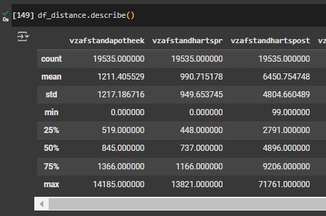
Using the Pandas .describe() function, we can store the values we need to calculate the Z-score for each data point.
Now we can find the z-score for each one using mean and standard deviation values obtained with Pandas. To do this, let’s name new variables for the mean and standard deviation values which will store those values for each feature:
means = df_distance.mean()
stds = df_distance.std()
Now that we have means and standard deviations, we can define the outlier range to filter using the following code:
outlier_mask_distances = ((df_distance - means) / stds).abs() > 3 This will make a selection that falls outside the allowed z-score per data point. This is a standard value to have (3 times the standard deviation). This will select all the outliers in the DataFrame. Now let’s invert the selection and only take the values that fall inside the z-score range:
non_outlier_mask_distances = ~outlier_mask_distances
df_distances_NoOutliers = df_distance[non_outlier_mask_distances.all(axis=1)]
The new DataFrame with no outliers are now saved in a new variable called df_distances_NoOutliers. To verify that you have removed the extreme values, you can print the following:
print('original distances dataframe:', df_distance.shape[0])
print('the new distances dataframe without outliers:', df_distances_NoOutliers.shape[0])
Features Data Distribution Visualization
We will examine the data distribution using the Box Plot graph method. Let us create two plots: first with the outlier data, the second with the outliers removed. This will give us a comparison of the extreme values after the data cleaning.
To create the original data distribution using box plot, use plt.boxplot(df_distance)
Then, save the y-axis limit to compare the before/after using this function: original_y_limits = plt.gca().get_ylim()
Give your plot a title: plt.title(‘Original Data with Outliers’) then finally show the plot. Note the extreme values here.
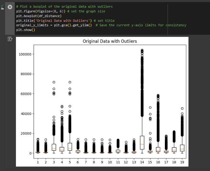
# Plot a boxplot of the original data with outliers
plt.figure(figsize=(8, 6)) # set the graph size
plt.boxplot(df_distance)
plt.title('Original Data with Outliers') # set title
original_y_limits = plt.gca().get_ylim()  # Save the current y-axis limits for consistency
plt.show()
Data Distribution After Outlier Removal
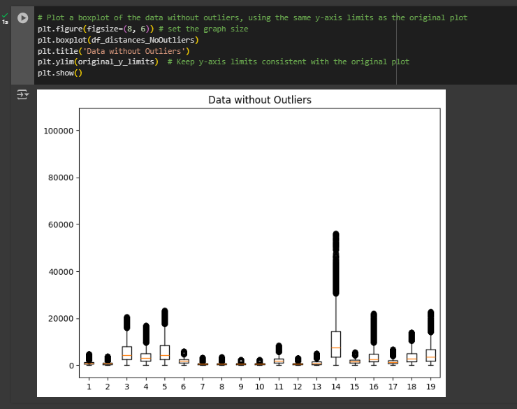
Now let’s run the same plot but on the new DataFrame with the outliers masked out.
# Plot a boxplot of the data without outliers, using the same y-axis limits as the original plot
plt.figure(figsize=(8, 6)) # set the graph size
plt.boxplot(df_distances_NoOutliers)
plt.title('Data without Outliers')
plt.ylim(original_y_limits)  # Keep y-axis limits consistent with the original plot
plt.show()
The distribution of the data will change with the removal of the extreme values so the box plot will look different. depending on the limit you set for the outlier mask, currently it’s set to 3 multiplied by the standard deviation (std) but you can change it to lower or higher number to include less or more from the data to remove.
Your new DataFrame that has the outlier removed are now called df_distances_NoOutlier.
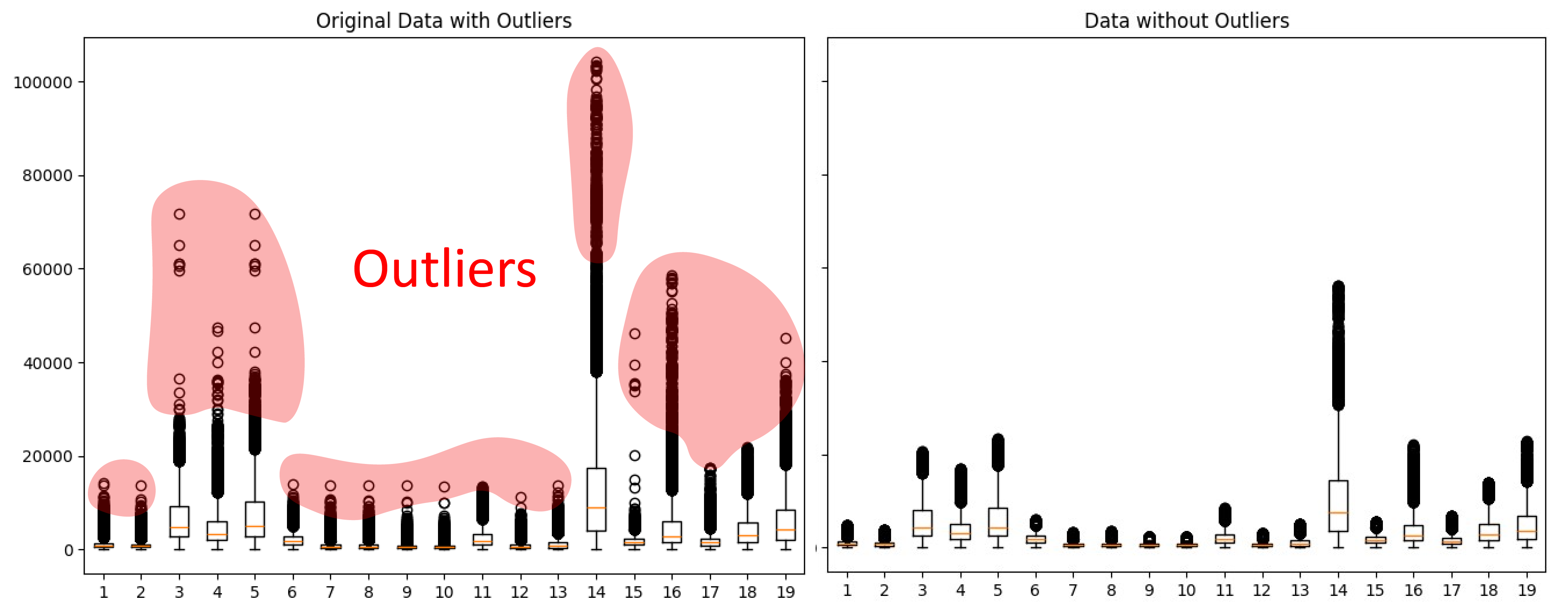
Here is the entire code below from the first step to identify the outlier range, creating the z-score mask and making a new DataFrame with outliers removed:
# Select columns with "vzafst" in their names, indicating distance features
distance_features = df_selection_removed.filter(regex='vzafst').columns

# find the mean and standard deviation of each feature
means = df_distance.mean()
stds = df_distance.std()

# find the outliers and create a mask
outlier_mask_distances = ((df_distance - means) / stds).abs() > 3

# apply mask to remove outliers from dataset
non_outlier_mask_distances = ~outlier_mask_distances
df_distances_NoOutliers = df_distance[non_outlier_mask_distances.all(axis=1)]

# print results of cleaning dataset from outliers
print('original distances dataframe:', df_distance.shape[0])
print('the new distances dataframe without outliers:', df_distances_NoOutliers.shape[0])
Data Normalization
Normalization of the data is a common technique in machine learning in the pre-processing step. As we have seen in the previous graphs, the features’ ranges vary greatly from one another, some features have maximum value of 500 while others 50000. Some machine learning algorithms will not work properly without normalization.
Also known as min-max normalization expressed as follows:
Where:
- X is the original value
- X^’ is the normalized value
- Xmin is the minimum value
- Xmax is the maximum value
The outcome of this operation will turn the feature from whatever minimum and maximum value into a new range from 0 to 1 float values.
To apply data normalization for your DataFrame, we will use Pandas. Let’s assign a new variable for the DataFrame to back to a simple df_clean variable”. And calculate the normalized values in the DataFrame:
df_clean = df_distances_NoOutliers
normalized_df = (df_clean-df_clean.min())/(df_clean.max()-df_clean.min())
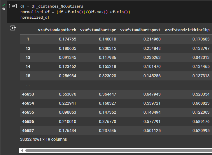
Now the DataFrame is normalized. To verify, you can view by entering the name of the variable in a new code field and run it; or plot the range using box plot method.
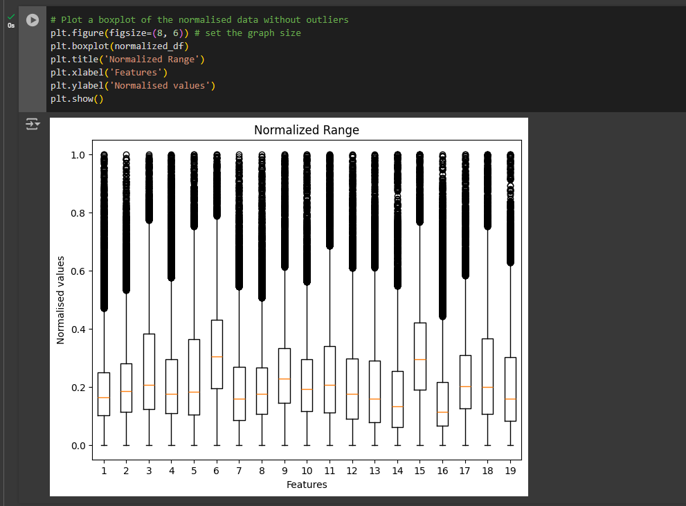
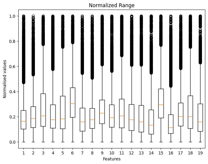
Next we will plot the normalized range after the normalization step. We will use the box plot similar to the previous step:
plt.figure(figsize=(8, 6)) # set the graph size
plt.boxplot(normalized_df)
plt.title('Normalized Range')
plt.xlabel('Features')
plt.ylabel('Normalised values')
plt.show()Preprocessing Datasets 6/7
Conclusionlink copied
In this tutorial, you learned the fundamentals of data cleaning/pre-processing. There are many different strategies for preparing different features. In here, we covered how to check if your data contains missing or NaN/null values. We also showed how to visualize the distribution of the data, select/remove features, detect outliers, and normalize data.
Exercise file
You can download the full Jupyter notebook here, with the complete code. The additional information of the dataset can be found in the first chapter.
Preprocessing Datasets 7/7
Useful Linkslink copied
Linked tutorials
You can find more information on the theory of using big data for research and the importance of data cleaning in the workshop ‘Pre-processing data for ML purposes’. This terminology page also provides information on outliers and normalisation.
Follow up tutorials
If you want to start using a dataset, the next step is to use the dataset for ML purposes.
External links
Here you can find the official website of the used dataset for this tutorial and websites to find a dataset for your own research or experiment.
Write your feedback.
Write your feedback on "Preprocessing Datasets"".
If you're providing a specific feedback to a part of the chapter, mention which part (text, image, or video) that you have specific feedback for."Thank your for your feedback.
Your feedback has been submitted successfully and is now awaiting review. We appreciate your input and will ensure it aligns with our guidelines before it’s published.
