Single-Criteria Optimization With Galapagos and Ladybug
-
Intro
-
Ladybug File Setup
-
Sunlight hours analysis
-
Single Criteria Optimization – the use of Galapagos
-
Conclusion
Information
| Primary software used | Ladybug |
| Course | Single-Criteria Optimization With Galapagos and Ladybug |
| Primary subject | Analysis & simulation |
| Secondary subject | Climate analysis |
| Level | Beginner |
| Last updated | December 19, 2024 |
| Keywords |
Responsible
| Teacher | |
| Faculty |
Single-Criteria Optimization With Galapagos and Ladybug 0/4
Single-Criteria Optimization With Galapagos and Ladybug
In this tutorial we are going to use the Ladybug plugin for shadow analysis.
Grasshopper is a platform which provides a platform for a range of simulation and analysis tools, in support of the Architectural design process. A range of plugins for Grasshopper are available which can be found on the Food4Rhino website. One of the plugins which is widely used is the Ladybug plugin. The plugin uses Energy Plus Weather files which can be selected based on location and downloaded contain weather data of the selected location.

Single-Criteria Optimization With Galapagos and Ladybug 1/4
Ladybug File Setuplink copied
For this tutorial we are going to use a Grasshopper file containing a setup for calculating the amount of shadow projected on a specific object. This example file will provide the option of loading a local (the Hague) Energy Plus Weather file containing a range of weather-related data which can be used in combination with the wide range of simulation and analysis options. A simplified location Rhino file is added where the terrace and roof can be imported.

For this tutorial we are going to use a Grasshopper file containing a setup for calculating the amount of shadow projected
Important: the example file is divided into 5 groups. We will discuss what each group does and how you can construct it yourself.
Group 1: Import Weather File [explanation of the example file]
Import Weather file:
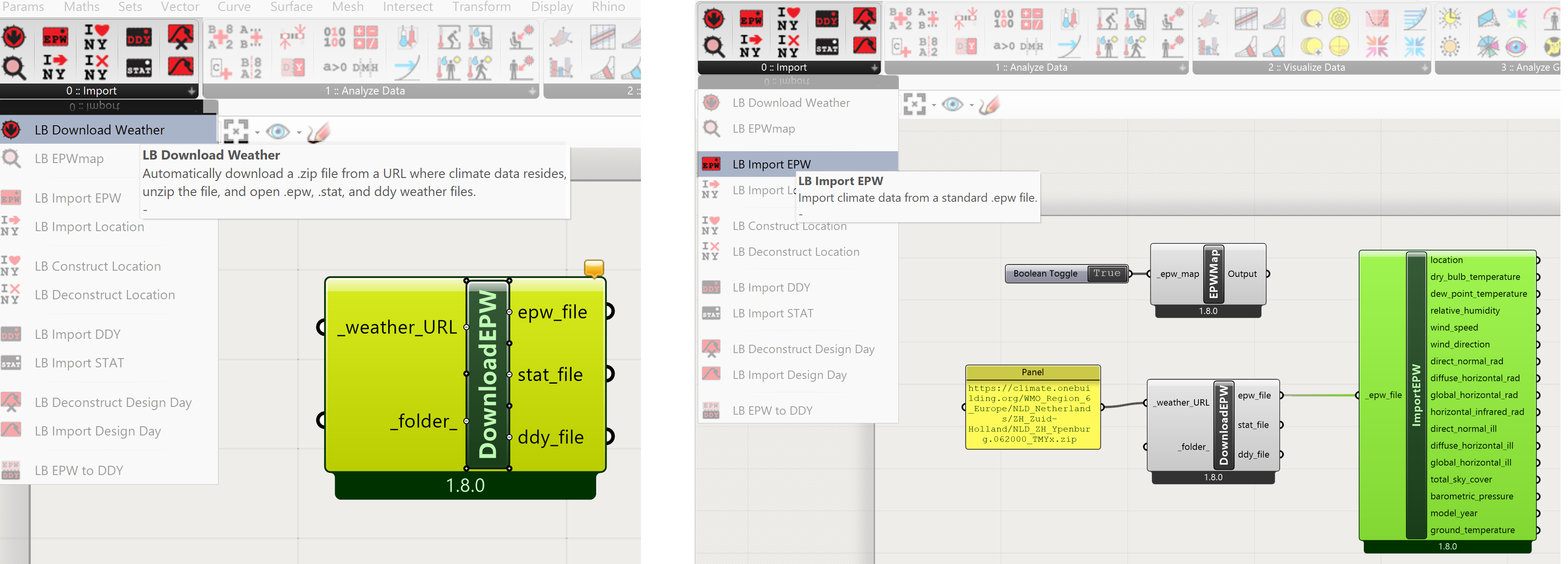
This group will allow you to get the correct EPW file. The Energy Plus Weather file is a file which contains weather data of a specific location. To make sure you collect the correct location data you can use a map with all the locations providing EPW file data.
The LBEPWmap component will give you access to the online map, where you can select the correct location for your EPW file.
To open the map, connect a Boolean parameter:
And double click on Boolean parameter to open the map.

Select the correct location and copy the link into a panel:
To download the correct EPW file we use the LB Download Weather component.
The panel containing the link is connected to the Weather_URL input of the LB Download Weather component. With this connection made, the data can be accessed with a variety of options.
Group 2 and 4: Creating Sun Path [explanation of example file]
Creating a Sun Path
The Sun Path component will generate a Sun path schematic based on the location of the EPW file. We need this setup because we are going to analyze in this tutorial the shadow effect of a roof on a terrace. The correct path of the sun is there for essential. To open the Sun Path component we go to LB SunPath.
The SunPath Component has a range of inputs.
North: This refers to the orientation of the Rhino location file. The provided Rhino location file has a 60 degree angle difference between the y axis and the North direction. Hence we connect a number slider or a panel with a 60 value with the North input of the SunPath component.
Location: We can use the output location information of the importEPW component for the Location input of the SunPath component. The EPWdata will provide the correct sun angles during the year.
HOY’s: Hour of the year input can contain two kinds of input. An input defining a single moment in time by the definition of a single hour, day and month. The sun will provide the correct angle on this specific time. The Ladybug>>Analyze Data>>LB Calculate HOY component has 4 inputs which can be defined with a Number slider. It is also possible with the HOY’s input to generate a calculation over a period of time. In that case we need a Ladybug>>Analyze Data>>LB Analysis Period component. Again, the inputs of the LB Analysis Period component can be defined with number slider.

- The next two inputs we can keep as they are ( DL_saving and Solar time)
- The Center_pt input can be relevant if the sunpath is not correctly located. However, the example files are correctly located so no change is needed.
- Scale : This allows us to scale the Sun Path. In this case we are going to use a factor of 5 scale. For this we couple a Number slider to the Scale input and set it to 5.
- The rest of the inputs we will not use for this tutorial.

Group 3: Direct Sun Hours [explanation of example file]
Analyzing the sun hours
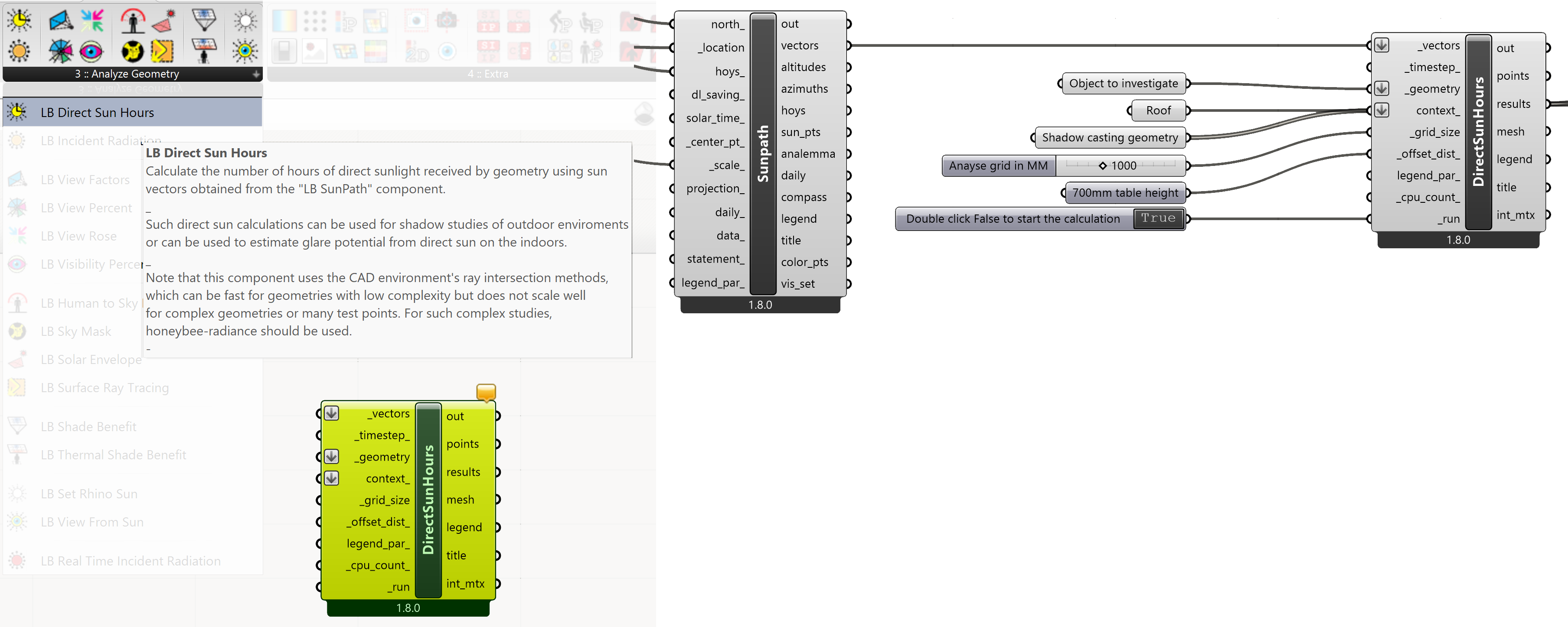
To examine the amount of sun hours on the terrace we use the Ladybug>> Analyze Geometry>>LB Direct Sun Hours component.
This allows us to investigate how much sun is reaching the terrace at a certain time or period. The LB Direct Sun Hours component has several inputs:
- Vectors: This refers to the vectors of the sun in relation to the location. This value is generated by the Sun Path component with the vector output. These can be connected.
- Timestep: for now we leave it as it is.
- Geometry: This is the geometry to be investigated. In this tutorial it will be the terrace. A Brep parameter called Object to Investigate is already linked to the Geometry input. Right click on the Object to Investigate node and select Set one Brep if the terrace consists of 1 part or Set Multiple Breps if the terrace consists of multiple parts.
- Context: This is connected to two Brep parameters. One is called Roof. This Roof parameter will be connected to the roof geometry. Right click on the Object to Investigate node and select Set one Brep if the roof consists of 1 part or Set Multiple Breps if the roof consists of multiple parts. The second Brep is called shadow casting geometry. The location can be selected and coupled to the Shadow casting geometry Brep by right clicking the Brep and select Set Multiple Breps. If you use the provided Rhino and Grasshopper file, the connection is already made.
- Grid size: The grid size is the size of the analysis grid – we can set this to 1000. This will generate a grid with the size of each grid element of 1000 by 1000 mm. The smaller the number the more grid elements are generated and the accuracy of the analysis increases. Each square meter will be analyzed if it receives sunlight.
- Offset_dist: Offset distance is the height of the grid in relation to the surface. In this case it is 700mm because we don’t measure the sun on the floor but at the height of a table which is about 700mm high.
- Ledgend_par: we keep as is – allows for customization of the legenda
- CPU_Count: we keep as is _ allows the selection of the amount of cores of the CPU dedicated to the calculations.
- Run: We connect a Parameter>>Input>>Boolean Toggle parameter to it. Double click on the Boolean Toggle parameter to switch the process of calculation off or on.
The model is set up and ready for use.
Single-Criteria Optimization With Galapagos and Ladybug 2/4
Sunlight hours analysislink copied
For this tutorial we are going to use two files which you can download at the start of the Ladybug File Setup chapter. The Grasshopper file contains the above explained analysis model. The Rhino file is a simplified version of the location. We use this simplified version so the light calculations needed for this analysis are faster.
Deciding when the terrace is open
What we are going to do is to analyse how much of the terrace is in the sun when the terrace is open to the public. Therefore you need to decide what period of the year the terrace is open and when it closes. Or it might be the full year open.
What might help with the decision when to open and close the terrace is a readout of the mean temperature over the full year from the EPW file.
Find the component LB Hourly Plot
This component will visualize the temperature range over the full year. Connect the Dry Bulb Temperature output of the Import EPW component to the Data input of the Hourlydata Component.
Use a Point component
The point component is used to define the location of the Plot. Right click on the Point component and select the Set one Point in option list. Place the point at a location where the Plot should be. This plot gives the mean temperatures during a year.

Based on this visualisation you can decide when the terrace could be open. Keep in mind the values are averages over several years, so events like heatwaves are averaged out.
Shadow analysis
For this tutorial we are going to use an unlikely openings period from 3-february 8.00 till 9- November 23.00. To get an idea where potential problems might occur with too much shadow or too much sun, we need to understand the use of the terrace. In the summer, some shade on the terrace at 14.00 might be preferable due to the summer heat. However, in the spring a terrace fully baking in the sun might be preferable due to the lower temperatures. We will investigate this later . First, we want an overview of the shadow casting roof and surroundings on the terrace.
We import only the terrace and the roof in the provided simplified location file. The Grasshopper script for the roof can be copied and pasted into the provided Grasshopper script.
- We connect the terrace to the Object to investigate parameter by right clicking on the parameter and select Set one Brep from the option list. The Object to investigate is the Geometry input for the Direct Sun Hours component.
- We connect the output of the designed roof in Grasshopper to the Roof parameter connected to the Context input of the Direct Sun Hours component. What simplifies the connection is to put the output of the designed roof into a Parameter>>Geometry>>Surface component.
- We activate the calculation by double clicking on the “Double click False to start the calculation” parameter.
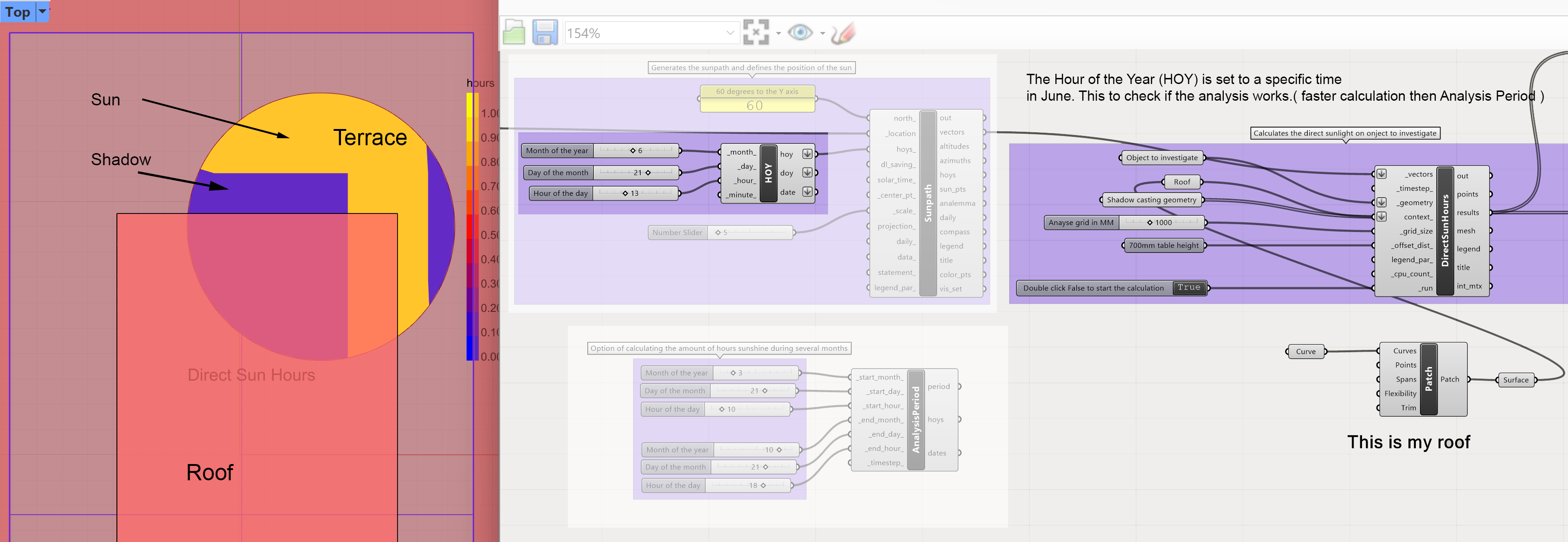
Note: if you expect to see sun on your terrace but everything is in the shadow, then it might be that the surface is upside down. You can correct this by selecting the terrace and type Flip in the Rhino command line.
Now that your geometry is connected,
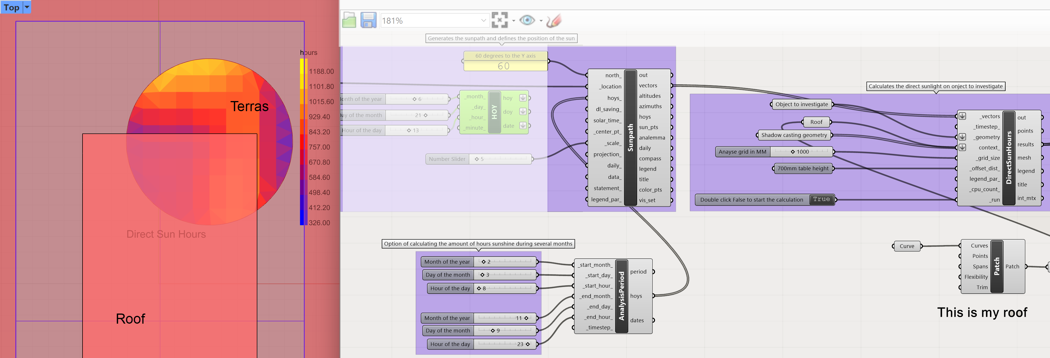
- connect the Analyse Period with the chosen settings for the period to the HOY’s input of the SunPath component.
- The result is a gradient of colours. The more yellow the more often the Sun will reach this spot during the year. Define the trouble spots on your terrace and device a strategy to make parts of the roof more parametric so relevant parts of the roof can be easily adjusted to enhance the distribution of shadow and sun light on your terrace.
Single-Criteria Optimization With Galapagos and Ladybug 3/4
Single Criteria Optimization – the use of Galapagoslink copied
In the previous part of the chapter, we looked how we can simulate the amount of sunlight on the terrace for a specific point in time or during a period of time. The outcome gives the designer insight on how the roof and its surroundings influences the amount of direct sunlight on the terrace. The surroundings are fixed, however the roof can be adjusted to support a more desired amount of direct sunlight on the terrace. This adjustment can be done by hand, by changing the roof – make a light calculation and see if the adjustment made it better. By doing this multiple times a solution might presents itself which gets close to an optimal solution. This can take quite a lot of time if you have a complex setup. For cases like this an AI might help to find an optimal solution for one or multiple criteria, for example the amount of sunlight on a terrace.
In this first part of the use of optimization components we use a single criteria optimization. That means that the algorithm will automatically search for one optimum for a single criterion. This criterion will be that the terrace should be 50% in direct sunlight at 13.00 on 31 July. This provides enough shade during high summer when the temperature might be too high to sit in the full sun.
Setup file for optimization
We are going to use the Galapagos component to search for an optimal light condition on the terrace for a specific time.
For this setup to work, we need make sure of 3 things:
- A roof made in Grasshopper which can be parametrically changed in Grasshopper with the use of a set of number sliders. Think about move, rotate or scale the whole roof. Or distort the roof by modifying the curves the roof is generated from.
- The HOY set to the correct time and date.
- The Galapagos component with the correct settings
An adaptable roof is already made in the previous assignment. Make sure the number sliders are constraint with realistic values. If you move a corner point of the roof limit the amount of movement possible to for example +6 meters and -6 meter in Y direction. To set this limitation double click on the number slider and set the minimum and maximum value. Also make sure you don’t use decimals; this can make the search process for an optimum much longer in time.
Connect the output of your parametric roof output to the “roof” geometry input the Ladybug component LB Direct Sun Hours.
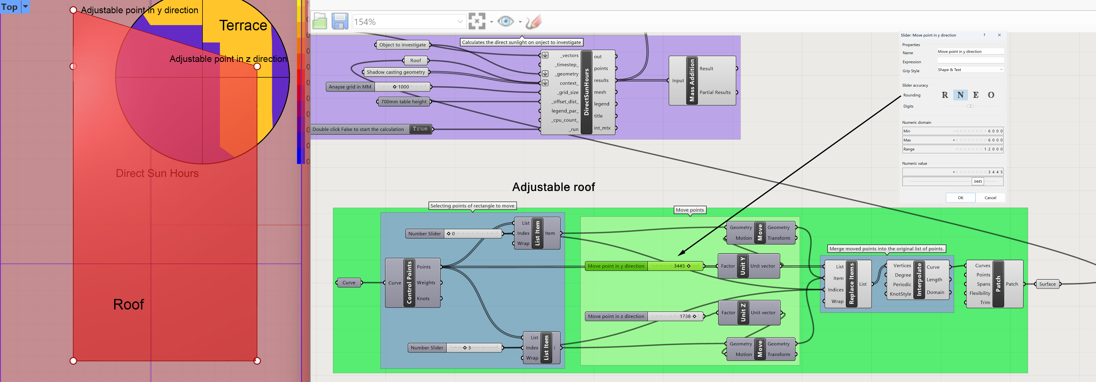
Defining Fitness Function in Galapagos
With the parametric roof connected to the roof input, the correct time and date must be set. We use the HOY component to set the correct time and date.
The last part is the placing the Galapagos component.
We have two inputs for the Galapagos component:
Genome: This is connected to the input for the number sliders we created to be able to adjust the roof shape. Galapagos shall change the values of the number sliders, during it search, in a smart way to find the optimal solution. To connect the number sliders to the Genome input, drag from the input of the Genome to the number sliders.
Fitness: fitness is the value Galapagos will be using to find the optimal solution. In this case 50% of the terrace must be in direct sunlight. For this we will use a calculation to determine what the 50% value should be. This will depend on the size of the terrace and the grid size used in the analysis. To get this data we count how many values are generated for the analysis. Each value represents a grid tile of your terrace. So half of the total amount of grid tiles have to be in direct sunlight. A grid tile receiving direct sunlight will have the value of 1, a tile who is in the shadow will receive the value 0 in this analysis. The target for the optimization can be read in the panel.
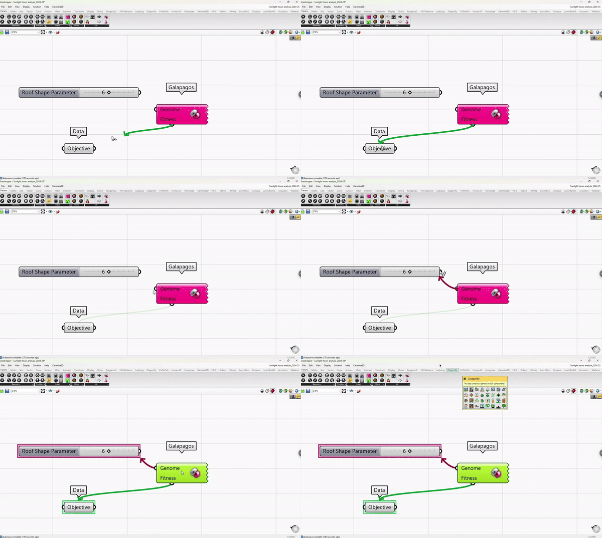
Defining your objective function is a key step in optimization. We can measure our objective by calculating the difference between the number of points receiving daylight from the total number of test points. We want half of the test points to be receiving daylight.
To know how many points are receiving daylight, we use the output Results of the Direct Sun Hours component gives us a list of 0 and 1, based on which of the grid tiles were in the shadow and which in the direct sunlight. If we add all the numbers, we get a value which represents the amount of tiles which are in direct sunlight, because the tiles in the shadow have the value 0.
Using the mass addition component, we can calculate the total value of points receiving sunlight by adding up all the 1 values from the results. Then using the list length component, this gives us the number of points in the list.
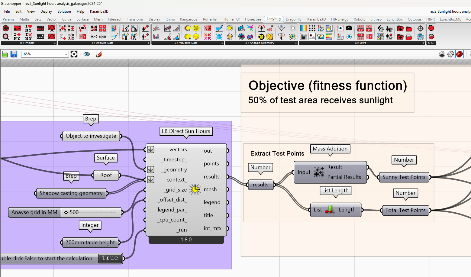
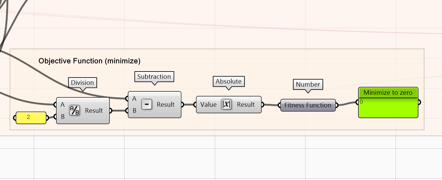
To calculate our objective function:
• First, we need to divide the list length by 2 which gives us the number of points (50%) of the test grid.
• Using this, we can subtract the number of points receiving sun with 50% of the points. If the result is 0, then half of the points are receiving sun. And the further away it is from zero, the further away the design is from the optimal solution.
• Then we use the absolute component to give us the absolute value. This is to avoid the algorithm to minimize in negative values.
• Then what you have is a value that is 0 when 50% of the surface receives direct sunlight.
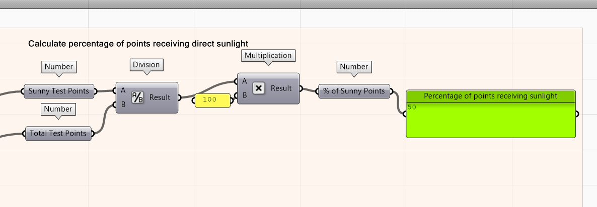
Using this same logic, we also can calculate the actual percentage:
- Divide the total number of sunny points by the total number of test points using the division component
- Multiply the number by a 100 using the multiplication component
- Plug the output into a panel to display
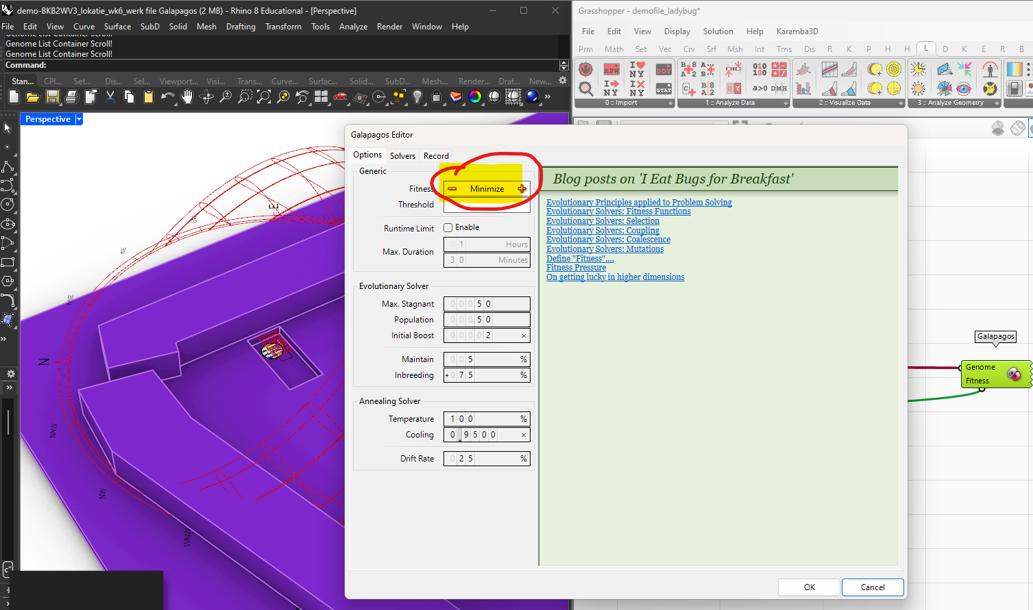
Setting up the Galapagos component.
If you double click on the Galapagos component, the settings menu opens. In this menu we set the values for the calculation. There are a range of settings:
- Fitness : this for whether you want to maximize or minimize the amount of shade. It can be set to a minimum or maximum value or a specific value. In our case, we want to minimize the value towards zero.
- The Threshold function is disabled with a target value.
- Run time limit: an option to limit the total calculation time. These can take quite a bit of time. Because the setup is relative simple we don’t need this option.
- Evolutionary Solver: the algorithm method that finds optimal solution for the design
- Max Stagnant: If the calculations constantly give the same result, this option will define after how many of the same values the calculation will be stopped. This prevents continuous calculations when the results will not improve the search for an optimum.
- Population: The size of the design variations the algorithm considers when running the solver. In this case we have 50 calculations.
- Initial Boost: This multiplies the first set of calculations to provide a good basis for the algorithm to make the selection to continue the calculations. If the population is set to 50 the initial boost will set the first set of calculations to 100.
- Maintain: defines how many of the original values can be used in the next generation of calculations. These values are analysed and used for a new set of values in the search for optimal values.
- Inbreeding: defines the amount of variation which can be generated during process. Too little is not good because it limits the search for the optimum. Too much can also be problematic because it can miss an optimal solution due to the amount of variations.
- Annealing solver: we keep as is.
The standard settings are a good starting point. If the calculations are getting too slow, you can decrease the Population size to 25.
To activate the calculation, go to the Solver tab and activate the Solver.
Important: because the calculations can take a while, the Rhino and Grasshopper file should always be saved before running the Solver.
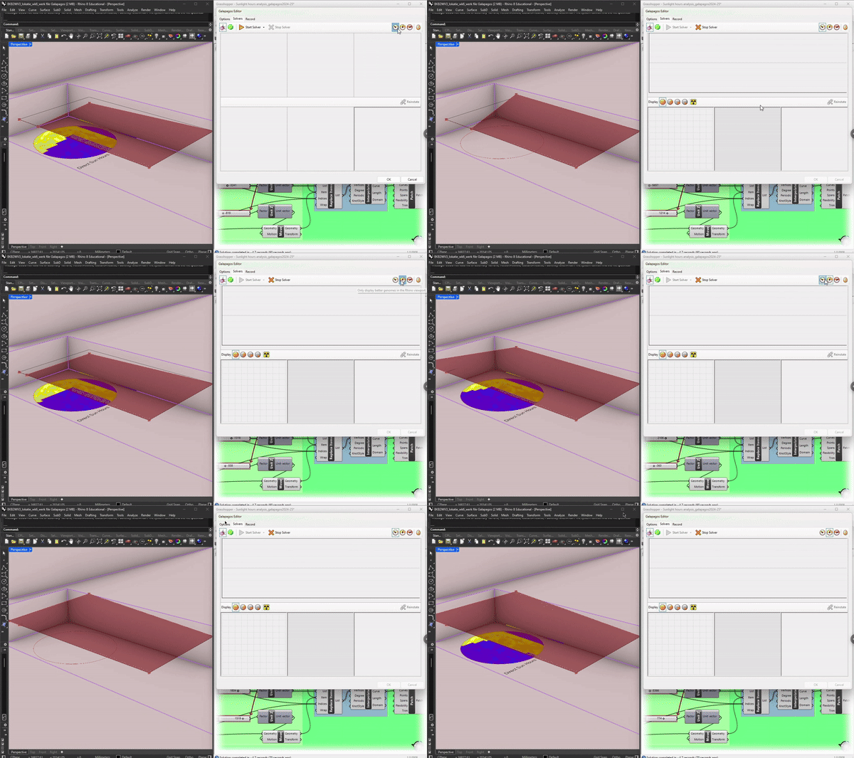
In the right top corner of the Solver menu there are 4 icons which define the display of the Grasshopper model. The first can be interesting because it will show the process of changing the grasshopper model in real time.
The display options in the left middle of the Solver menu shows the various amounts of Gnomes ( solutions) in the two other views.
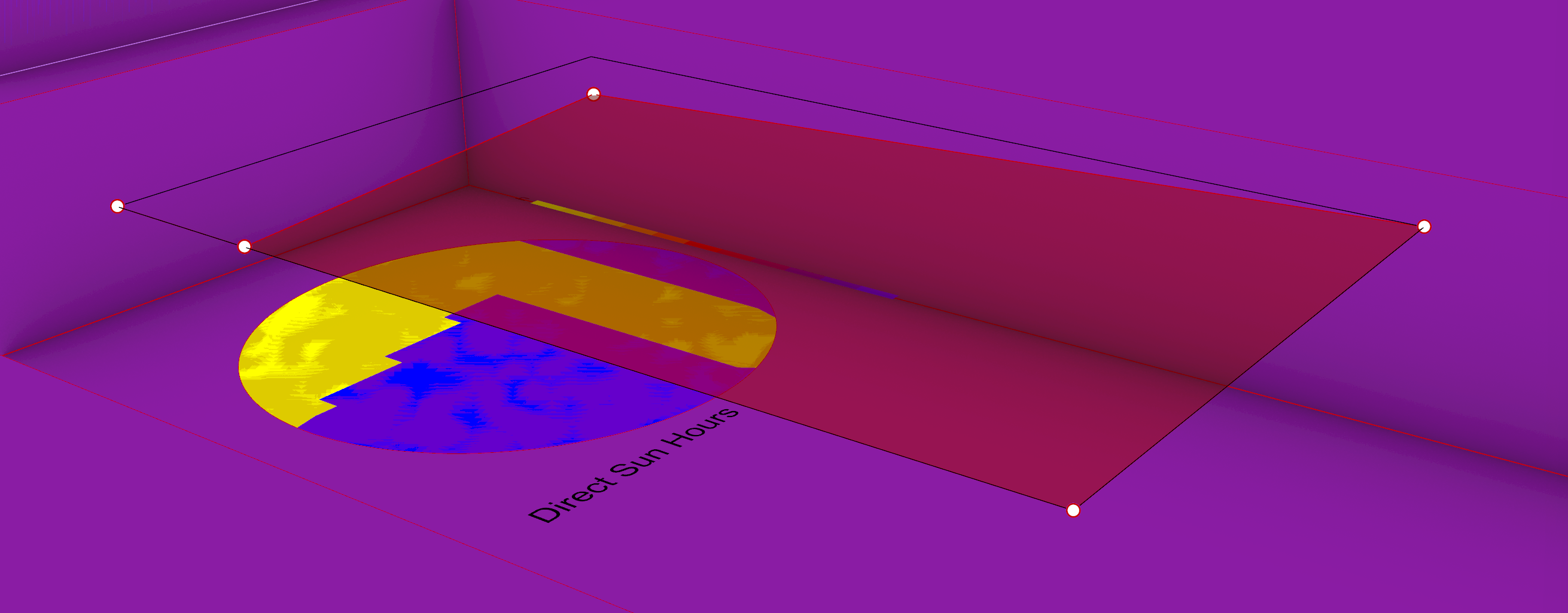
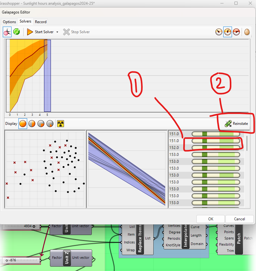
Once the analysis is done, you can re-instate design solutions by clicking on the green bars and then clicking on Reinstate. This can give you more control on which design option you pick while also getting an idea on the daylight/shade percent.
- Click on the green bar
- Click reinstate
Single-Criteria Optimization With Galapagos and Ladybug 4/4
Conclusionlink copied
You now have begun your climate analysis process by:
- setting up the climate model using Ladybug,
- connecting a parametric geometry, your roof, to investigate the shadow effect
- setting single the Galapagos component and defining your fitness (objective function) and genomes (the geometry to adjust)
You can expand on this by adjusting the parameters that affect your roof for example. This now helps come up with more climate-responsive designs.
Relevant tutorials
Follow up tutorials
Write your feedback.
Write your feedback on "Single-Criteria Optimization With Galapagos and Ladybug"".
If you're providing a specific feedback to a part of the chapter, mention which part (text, image, or video) that you have specific feedback for."Thank your for your feedback.
Your feedback has been submitted successfully and is now awaiting review. We appreciate your input and will ensure it aligns with our guidelines before it’s published.
