Honeybee Energy Analysis with Open Studio
-
Intro
-
Design
-
Model Preparation
-
Compose the Program Type (Set Schedules & Energy Loads)
-
Compose the HB model for the Energy simulation
-
Create & Run the Open Studio simulation
-
Post-Processing the Results
-
Conclusion
-
Useful Links
Information
| Primary software used | Honeybee |
| Course | Honeybee Energy Analysis with Open Studio |
| Primary subject | Analysis & simulation |
| Secondary subject | Climate analysis |
| Level | Intermediate |
| Last updated | February 19, 2025 |
| Keywords |
Responsible
| Teacher | |
| Faculty |
Honeybee Energy Analysis with Open Studio 0/8
Honeybee Energy Analysis with Open Studio
Learn to use energy modelling tools in Grasshopper through the Honeybee plugin
In this tutorial you will learn how to set-up and run an energy analysis within Grasshopper utilizing Honeybee and Open Studio. This tutorial will guide you step by step to learn how to set the construction and program type, compose the HB room for an Energy simulation, create and run the simulation with Open Studio and finally. Post-process the results.
Honeybee Energy Analysis with Open Studio 1/8
Designlink copied
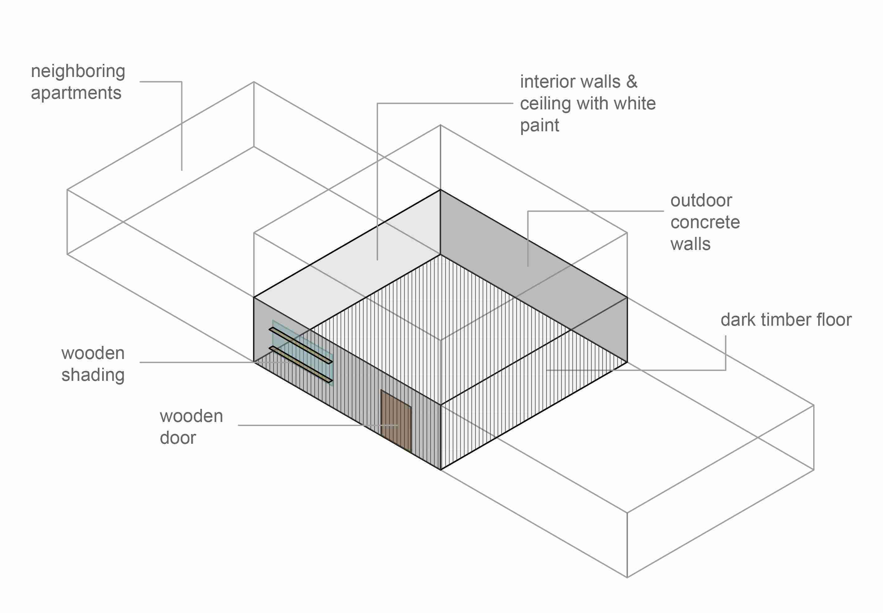
This example refers to a shoebox geometry of an apartment which is on the ground floor of a 2-storeys building. It has a rectangular plan of 10m*10m and it has a height of 3m.
The apartment has an entrance from the road with an opaque wooden door and has also one operable window facing the street. The window is shaded with wooden horizontal louvres. On the left and right side there are adjacent apartments, but on the back side it is not neighbouring any other apartment or building.
The exterior walls are made of concrete in light grey colour. The slabs are also made of concrete, and they are painted in white colour on the bottom side (ceiling). On the top part (floor), they are covered in darker coloured timber. The interior walls are made of plywood and covered also in white paint.
Given that the example model refers to a small single-family apartment, we are going to assume that, on weekdays, it is mostly occupied during the afternoon hours, whereas, on weekends and holidays, it is occupied all day long. Regarding the HVAC systems, we are going to assume that the apartment has only natural ventilation and no mechanical ventilation or heating/cooling at all.
For this tutorial, the same example the room design is used as in the tutorial is used as in ‘Creating the HB model‘. Therefore, to continue with the Energy Analysis you should have, firstly, created an HB model based on your design following the steps described in the Creating the HB model tutorial.
Honeybee Energy Analysis with Open Studio 2/8
Model Preparationlink copied
To run the energy simulation with Open Studio, you should, firstly, define the thermal properties of the materials that compose each building component. Through creating the Construction Sets, the material thermal properties will be assigned to the different elements. Additionally, the weather data need to be imported.
Opaque Materials & Constructions
Before following on with the Energy analysis, you should make sure that the relevant material properties are defined for each building element. In the steps that follow you will learn how you can assign material properties to the HB model. To do so, first the radiance modifiers per material are created, then the modifier subsets are created per face from which the modifier set is created. Lastly, the modifier set is assigned to the HB model after which you can visualize and check the modifiers.
For a more accurate Energy simulation, you should assign the values of the material properties for each material in the corresponding surfaces. Specifically, you should specify the material thickness, thermal conductivity, density, and specific heat.
- Material thickness [m]
- Thermal conductivity [W/m*K], which is the rate at which heat is transferred by conduction through a unit cross-section area of the material.
- Density [kg/m3], which is ….
- Specific heat [J/kg*K], which is the amount of heat needed to increase the temperature of 1kg of the material by 1K.
Opaque Material Properties
For all the material layers in each building element (e.g floor/ceiling/exterior walls/interior walls) a HB Opaque component needs to be created. Then the material name should be defined together with the specific heat, density, thermal conductivity and material thickness.
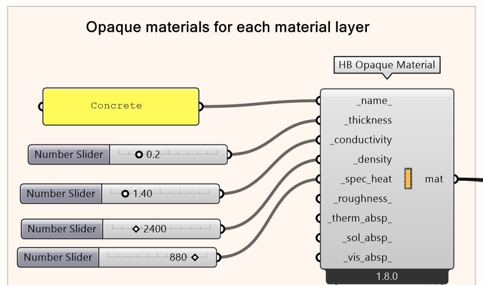
Create an HB Opaque Material component.
Create a Panel component to set the name of the material layer. Connect it to the ‘_name_’ input.
Create 4 Number Slider components to set respectively
Note: It may be the case that the same material is placed in different building elements in the model. If the material layers do not have the same thickness, then different HB Opaque Material components should be created for each of the different thicknesses.
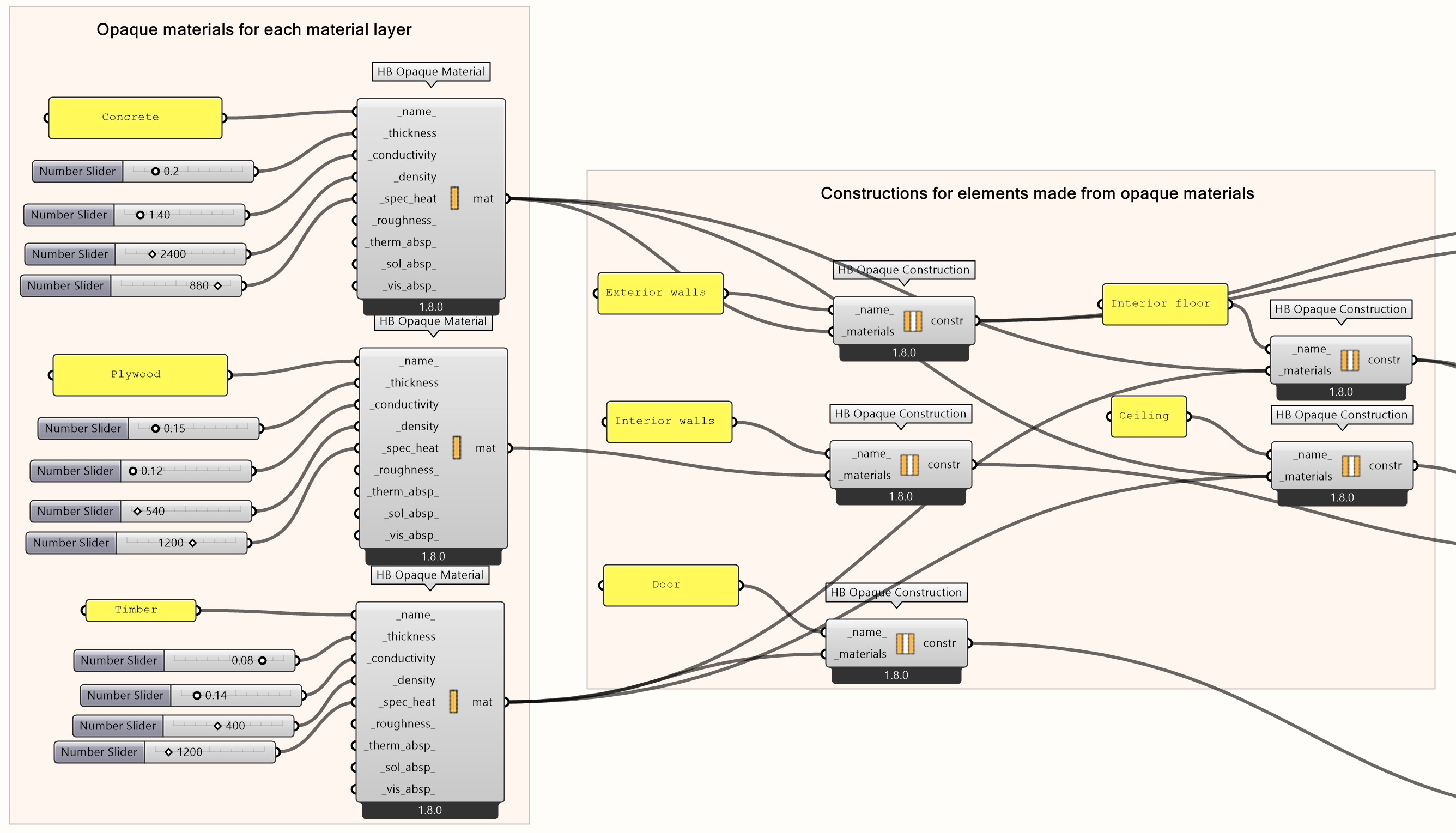
| Material Name | Thickness [m] | Conductivity [W/m2K] | Density [kg/m3] | Specific Heat |
| Concrete | 0.20 | 1.40 | 2400 | 880 |
| Plywood | 0.15 | 0.12 | 540 | 1200 |
| Timber | 0.08 | 0.14 | 400 | 1200 |
Table: opaque material properties for the example room
To implement this:
- Create an HB Opaque Construction component for each of the building elements.
- Create a Panel component to set the name of each element. Connect it to the ‘_name_’ input.
- For each of the material layers that compose the building element, connect the ‘mat’ result of the HB Opaque material to the ‘_materials’ input of the HB Opaque Construction component.
Note: in case one building element is composed of more than one material layer, you should connect them in order from the exterior to the interior layer. Therefore, the interior floor and ceiling should have as inputs the same material layers but placed in reverse order.
For this example, you should create 5 HB Opaque Construction components and set:
| Construction Name | Material 1 | Material 2 |
| Exterior Walls | Concrete | |
| Interior Walls | Plywood | |
| Door | Timber | |
| Interior Floor | Concrete | Timber |
| Ceiling | Timber | Concrete |
Table: opaque material constructions for example room
Window Materials & Constructions
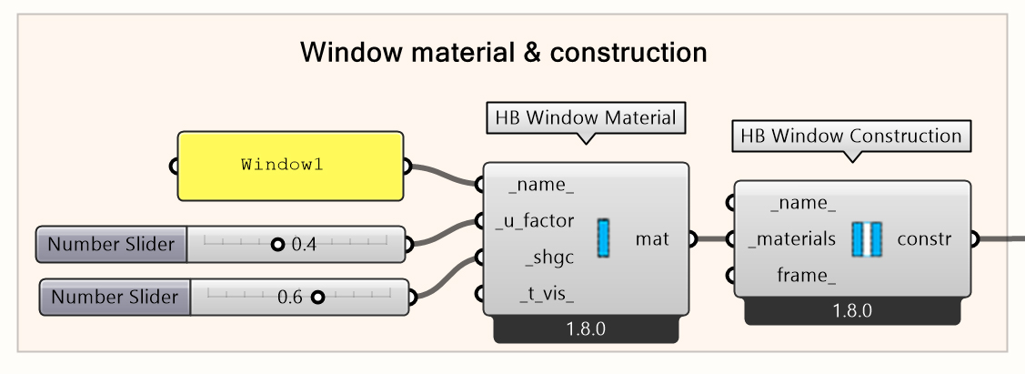
For the windows of the building:
- Create an HB Window Material component for each of the openings that you need to specify.
- Create a Panel component to set the name of the opening. Connect it to the ‘_name_’ input.
- Create 2 Number Slider components so as to set respectively
-
- U-factor (‘_u_factor’) – W/m2*K (defining how fast heat from hot air will pass through the glazing system).
- Solar heat gain coefficient (‘_shgc’) – defining how fast heat from direct sunlight will pass through the glazing system.
In this example, you should create 1 HB Window Material component and set:
‘_name_’: Window1, ‘_u_factor’: 0.4, ‘_shgc’: 0.6
Connect the material output ‘mat’ to the material input of HB Window Construction
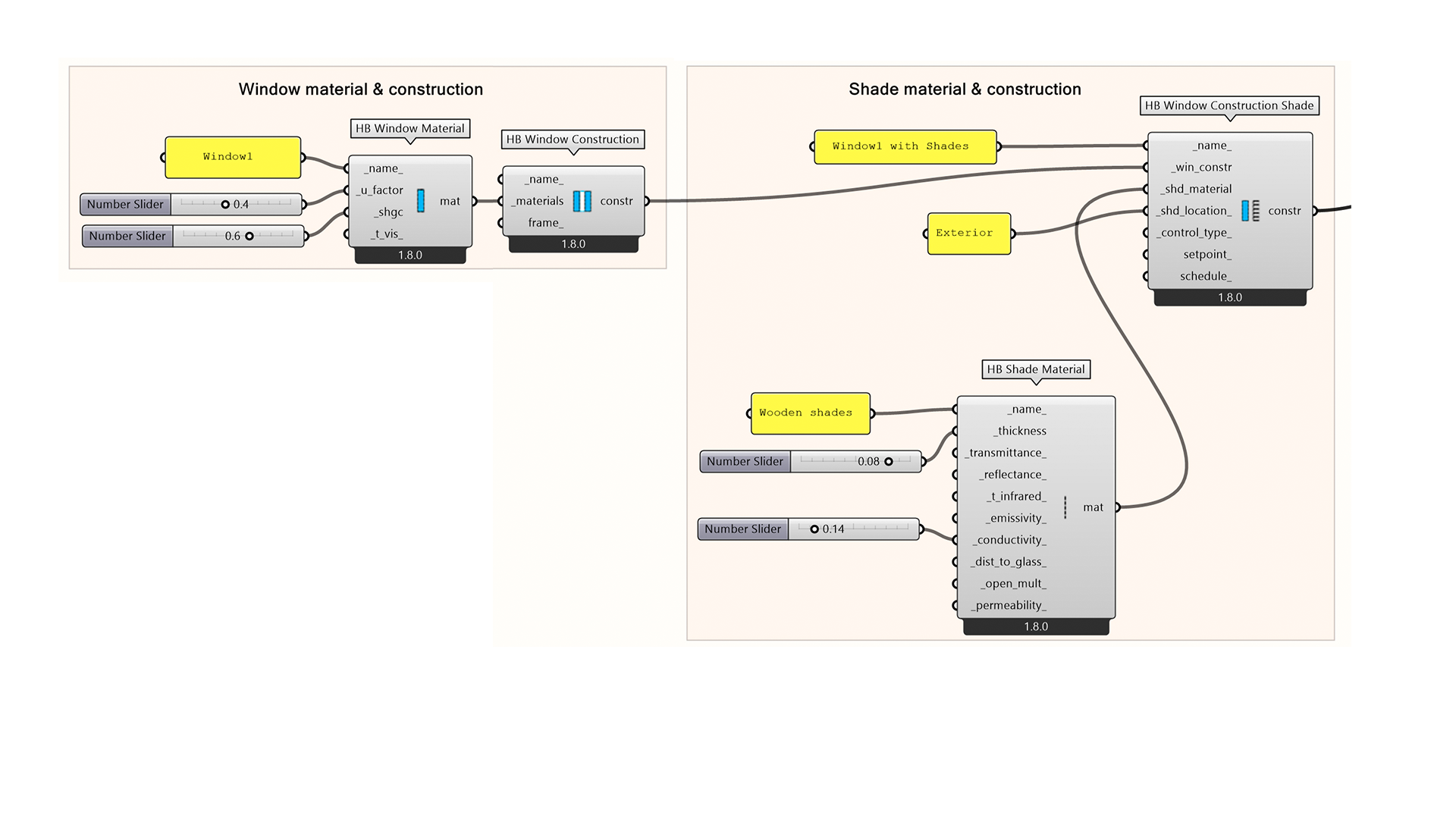
Shade Materials & Constructions
For the shades placed outside the windows of the building:
- Create an HB Shade Material component.
- Create a Panel component to set the respective name. Connect it to the ‘_name_’ input.
- Create 2 Number Slider components and set respectively:
-
- Thickness of the material layer (‘_thickness’) – m
- Thermal conductivity (‘_conductivity’) – W/m*K (how easy the material can transfer heat through its mass)
For this example, set: ‘_name_’: Wooden shades, ‘_thickness’: 0.08, ‘_conductivity_’: 0.14.
By browsing your mouse over the inputs, you can see which other values can be set.
Next, the construction component.
- Create a HB Window Construction Shade component.
- Create a Panel component to set the respective name. Connect it to the ‘_name_’ input. For this example, write Window1 with Shades.
- Connect the ‘constr’ result of the HB Window Construction component to the ‘_win_constr’ input.
- Connect the ‘mat’ result of the HB Shade Material component to the ‘_shd_material’ input.
- Then, create a new Panel component and connect it to the ‘_shd_location_’ input. Write Exterior to define that the shades will be placed on the outer side of the opening.
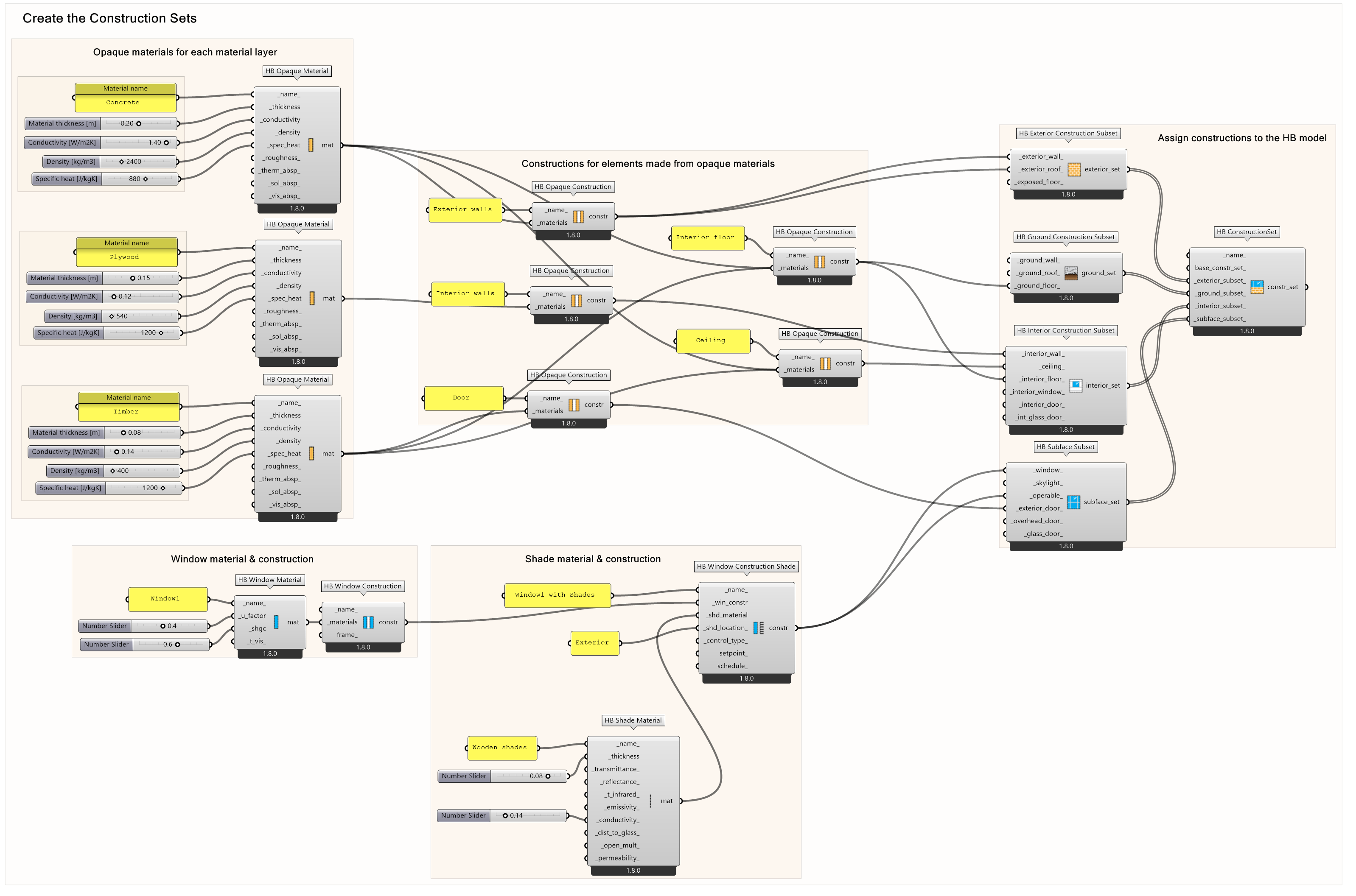
Assign Constructions to the HB Model
To assign the constructions to the HB model, you should create the Construction Subsets and the final Construction Set. The step to do so are:
Create:
- An HB Exterior Construction Subset component.
- An HB Ground Construction Subset component.
- An HB Interior Construction Subset component.
- A HB Subface Subset component.
- Connect the ‘constr’ result of the HB Opaque Construction and HB Window Construction Shade components to the respective inputs of the Construction subsets.
- Create an HB ConstructionSet component.
- Connect the results from the Construction Subsets (‘exterior_set’, ‘ground_set’, ‘interior_set’, ‘subface_set’) to the respective inputs of the ConstructionSet. Connect the ‘constr_set’ result of the HB ConstructionSet component to the ‘_const_set_’ input of the HB Room component as created in the following tutorial.
For background information on a HB room setup, review this tutorial:
Honeybee Energy Analysis with Open Studio 3/8
Compose the Program Type (Set Schedules & Energy Loads)link copied
Following assigning material thermal properties, the internal energy loads and their corresponding schedules, related to the occupancy of the space, should be set.
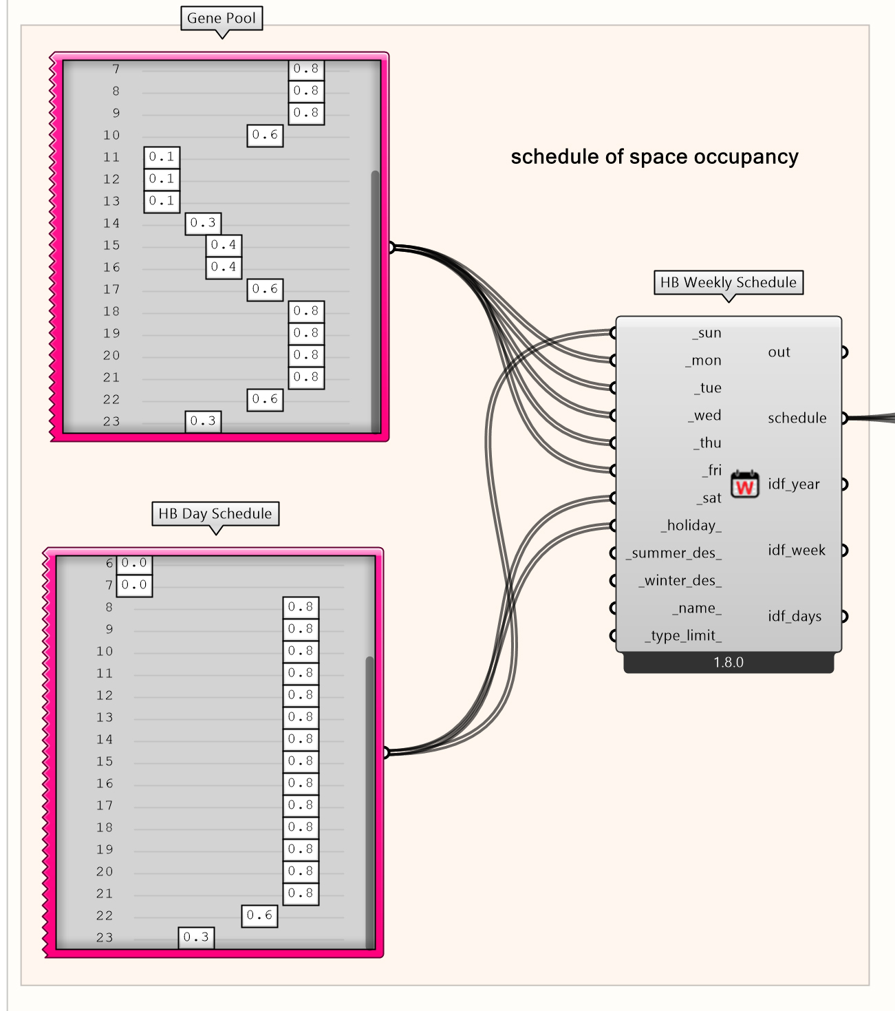
Occupancy schedules
In the Schedules subpanel, you can find different ways for creating a schedule.
However for this tutorial:
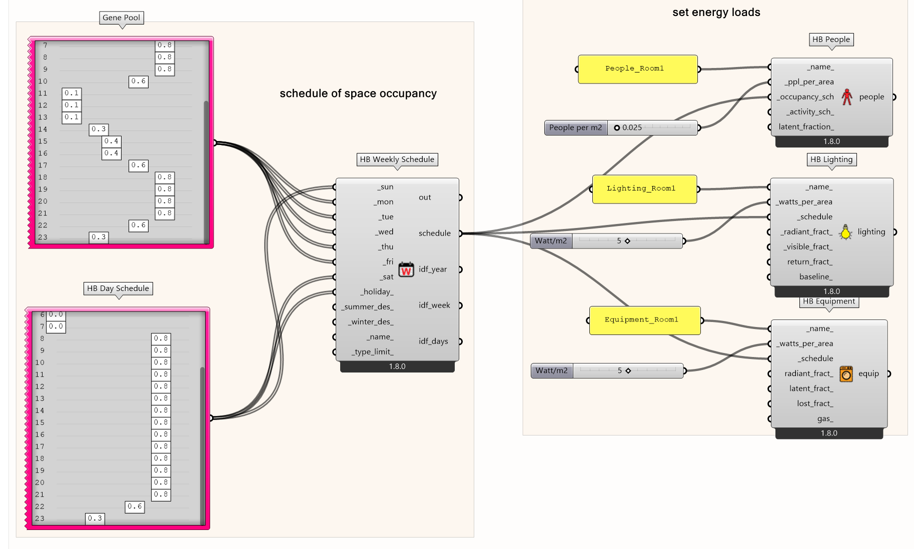
- Create an HB Weekly Schedule component.
- Create a Gene Pool component to set the values for the occupancy per hour regarding the weekdays and another Gene Pool component to set the respective values during weekends & holidays.
- Double-click in the Gene Pool components and set:
-
- Gene Count: 24 (the total number of hours per day)
- Decimals: 1, Minimum: + 0.00, Maximum: + 1.00
Important to note: The minimum and maximum values are set like this, because they refer to fractional values (proportion of occupancy per hour).
By moving the sliders of the Gene Pool, you can set the values for the different hours. Since the room is an apartment, you should set higher values in the early morning and afternoon hours, for the weekdays, and during the whole day for weekends & holidays (see image).
- Connect the Gene Pools to the respective day inputs on the HB Weekly Schedule component.
To visualize and check the schedules you have created:
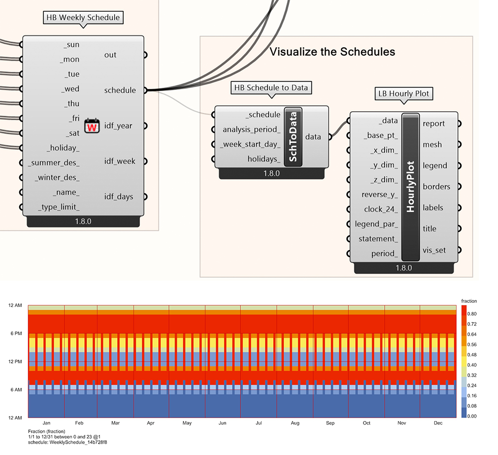
- Create an HB Schedule to Data component. Connect the ‘schedule’ result of the HB Weekly Schedule component to the ‘_schedule’ input.
- Create an LB Hourly Plot component. Connect the ‘data’ result of the HB Schedule to Data component to the ‘_data’ input. By clicking on the LB Hourly Plot component, you can see the resulting graph in Rhino.
Loads
In the Loads subpanel you can find the different energy loads that can be applied.
In this example we are going to add to the room:
A. Load of the number of people per m2 of area.
- Create a HB People component.
- Create a Panel component to set the ‘_name_’ input to People_Room1.
- Connect the ‘schedule’ result of the HB Weekly Schedule component to the ‘_occupancy_sch’ input.
- Create a Number Slider component to set the ‘_ppl_per_area’ input to 0.025 (value corresponding to an apartment).
- Connect the ‘schedule’ result of the HB Weekly Schedule component to the ‘_schedule’ input.
- Create a Number Slider component to set the ‘_watts_per_area’ input to 5 (value corresponding to a single-family apartment).
B. Load for the lighting power density in Watts per m2 of area
- Create an HB Lighting component
- Create a Panel component to set the ‘_name_’ input to Lighting_Room1.
- Connect the ‘schedule’ result of the HB Weekly Schedule component to the ‘_schedule’ input.
- Create a Number Slider component to set the ‘_watts_per_area’ input to 5 (value corresponding to a single-family apartment).
C. Load for the equipment power density in Watts per m2 of area.
- Create an HB Equipment component.
- Create a Panel component to set the ‘_name_’ input to Equipment_Room1.
- Connect the ‘schedule’ result of the HB Weekly Schedule component to the ‘_schedule’ input.
- Create a Number Slider component to set the ‘_watts_per_area’ input to 5 (value corresponding to a single-family apartment).
To connect them altogether:
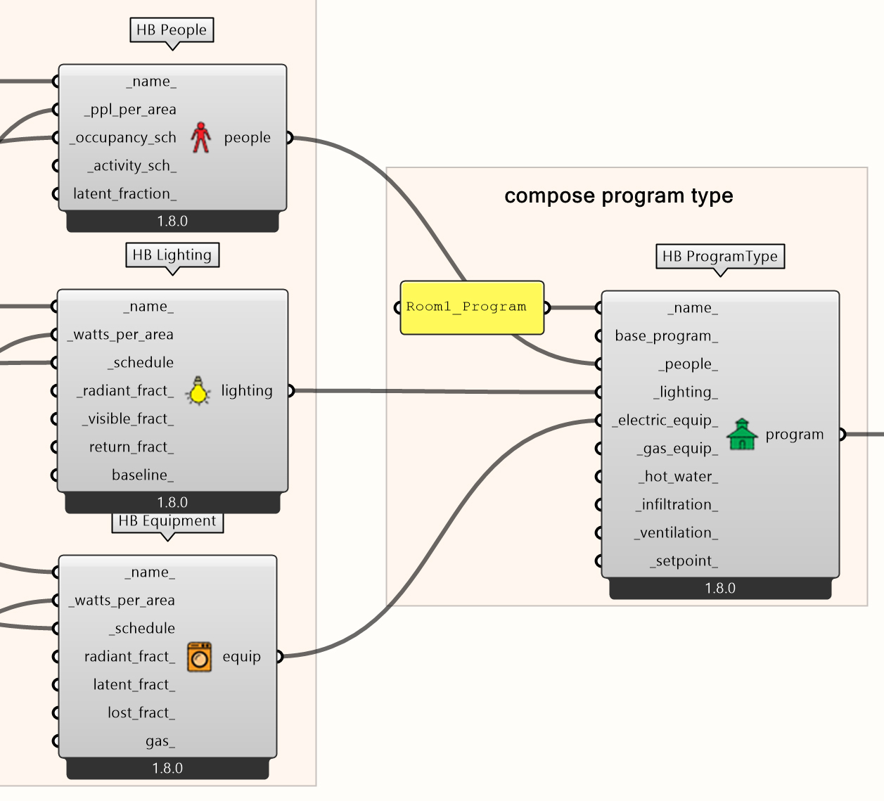
- Create an HB ProgramType component.
- Create a Panel component to set the ‘_name_’ input to Room1_Program.
- Connect the ‘equip’ result of the HB Equipment component to the ‘_electric_equip_’ input of the HB ProgramType component. Do the same for the ‘people’ and ‘lighting’ results respectively.
Important to note: The aforementioned refer to a detailed version of setting the Loads according to the occupancy Schedules. There are also simpler options, such as:
- HB Building Programs – You can add one of the existing programs based on the use of the building.
HB – Energy → Basic Properties → HB Building Programs
- HB Apply Absolute Load Values – You can add the absolute values per load without modifying them according to a schedule.
HB – Energy → Basic Properties → HB Apply Absolute Load Values
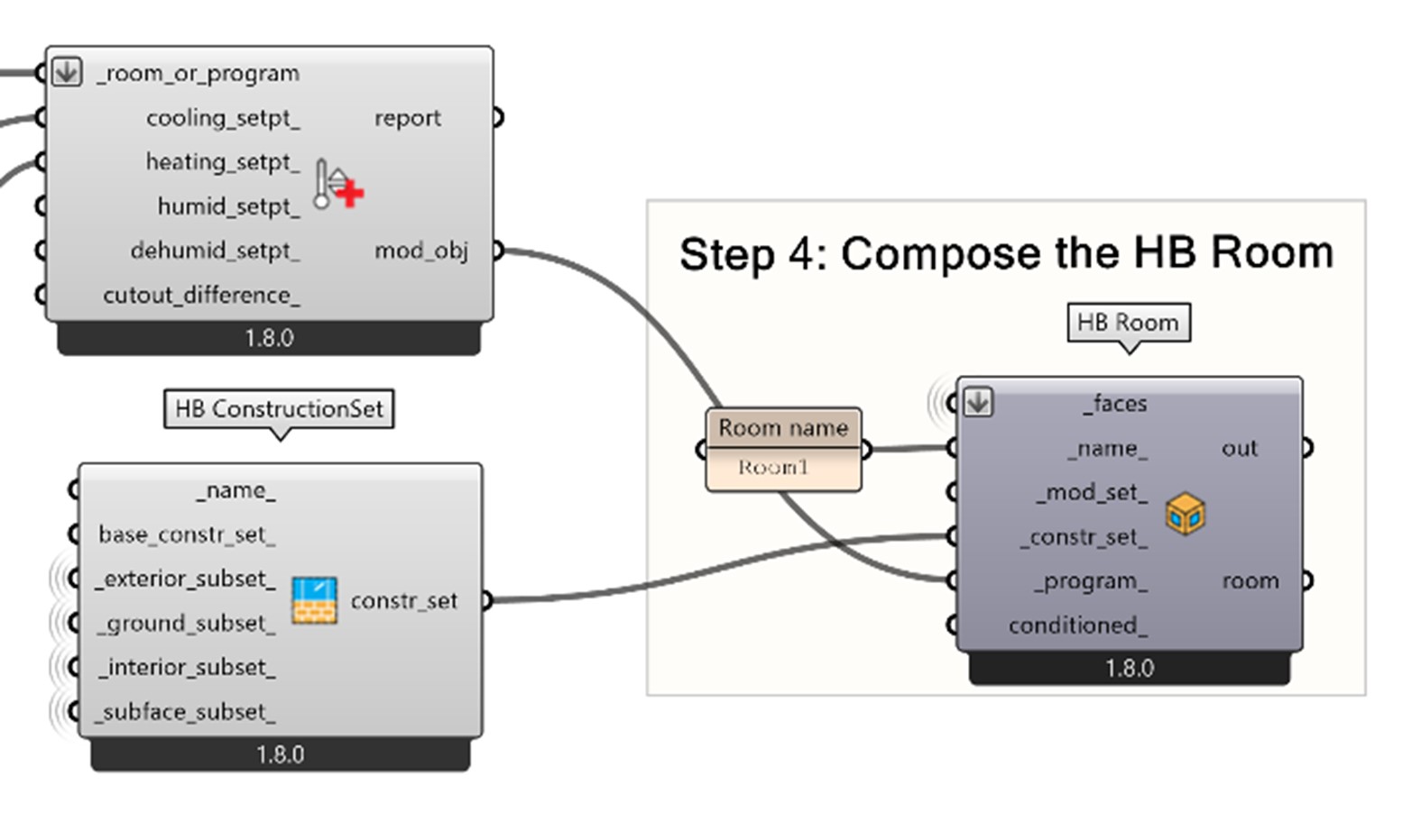
Next, setting up the heating and cooling setpoitns:
- Create an HB Apply Setpoint Values component to set the heating and cooling setpoints. These correspond to the temperatures below which heating will be needed and above which cooling will be needed respectively.
- Connect the ‘program’ result of the HB ProgramType component to the ‘_room_or_program’ input of the HB Apply Setpoint Values component.
- Create 2 Number Slider components and connect them to ‘cooling_setpt_’ and ‘heating_setpt_’ respectively. For this example, set the heating setpoint to 20 and the cooling setpoint to 27.

- Connect the ‘mod_obj’ of the HB Apply Setpoint Values component to the ‘_program_’ input of the HB Room component.
Honeybee Energy Analysis with Open Studio 4/8
Compose the HB model for the Energy simulationlink copied
There are multiple steps to prepare the HB model for the Energy simulation. These steps are:
- Assign Construction Set & Program type
- Assign Internal Mass
- Set Natural Ventilation Parameters
- Compose the HB Model
- Visualize & Check the HB Model
1. Assign Construction Set & Program Type
If you have not already done it during the previous 2 steps of this tutorial, you should connect the following parameters in the HB room:
- Connect the ‘constr_set’ result of the HB ConstructionSet component (as created in Model Preparation (Opaque Materials & Constructions)) in the ‘_constr_set_’ input of the HB Room.
- Connect the ‘mod_obj’ result of the HB Apply Setpoint Values component (as created in Compose the Program Type (Set Schedules & Energy Loads)) in the ‘_program_’ input of the HB Room.
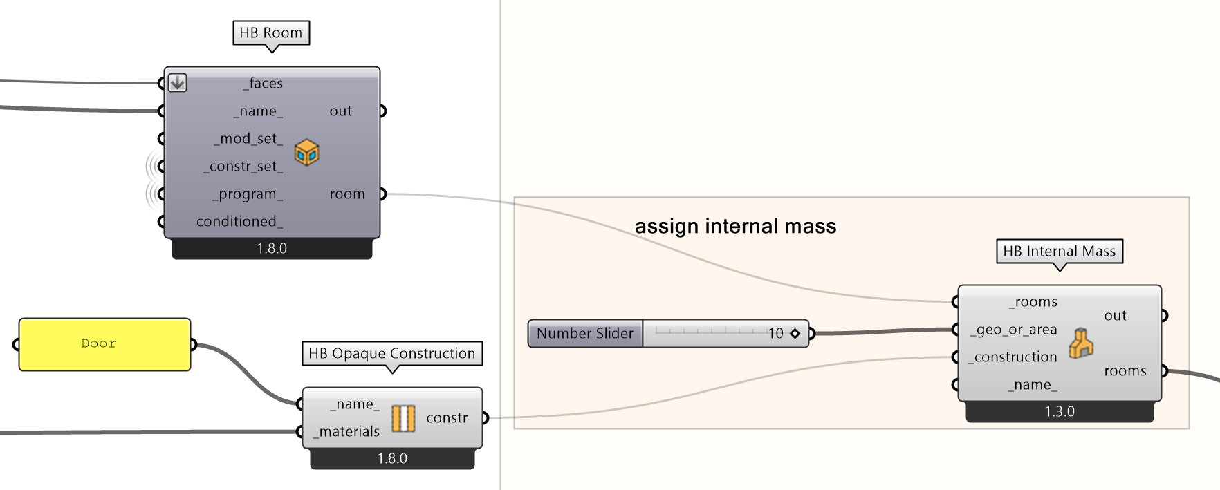
2. Assign Internal Mass
The internal thermal masses refer to the effect of furniture or other massive building components in the energy simulation. To assign internal mass to the HB model:
- Create an HB Internal Mass component.
In the ‘_construction’ input, connect the ‘constr’ result of the HB Opaque Construction component that corresponds to the material of the internal mass.
For this example, you should connect the result from the “Door” construction as created in Model Preparation (Opaque Materials & Constructions), since we are going to calculate the internal mass of wooden furniture.
Important to note: Each component corresponds to the internal mass of a specific material. If you want to calculate internal masses of more than one material, you should create different components.
- Create a Number Slider component to set the ‘_geo_or_area’ input, related to the surface (in m2) of the internal mass. In this example, you should set it to 10.
3. Set Natural Ventilation Parameters
Next step is to set the Natural Ventilation parameters for the room.
Important to note:
- To define which windows are operable, you should have set the ‘operable_’ input to True, when creating the respective HB Aperture. Otherwise, natural ventilation will not be calculated for these apertures.
- In this example, we are not going to calculate the mechanical ventilation. However, if you want to add it to your design, you can find the respective components on the subpanel.
HB – Energy → HVAC
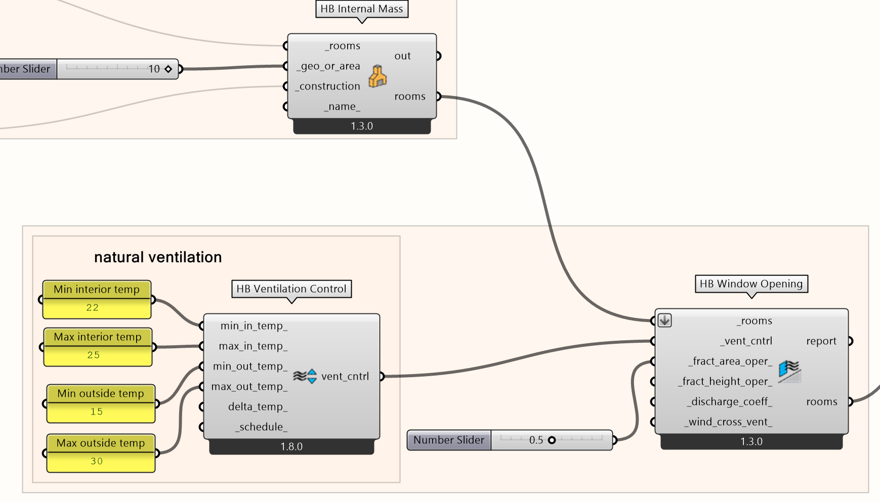
To set the Natural Ventilation parameters:
- Create 4 Panel components and set:
- Min interior temperature (‘min_in_temp_’): 22
- Max interior temperature (‘max_in_temp_’): 25
- Min outside temperature (‘min_out_temp_’): 15
- Max outside temperature (‘max_out_temp_’): 30
Important note: You should ensure that the temperature range for natural ventilation is well between the overall setpoints for heating and cooling of the room as set in Compose the Program Type (Set Schedules & Energy Loads). If they overlap, two contradictory functions (e.g. heating and natural ventilation bringing cold air from outside) may happen simultaneously. Thus, the min interior temperature of natural ventilation should be approximately 2 degrees higher than the heating setpoint and the max interior temperature should be 2 degrees lower than the cooling setpoint respectively.
Create an HB Window Opening component.
- Connect the ‘rooms’ result of the HB Internal Mass component to the ‘_rooms’ input.
- Connect the ‘vent_cntrl’ result from the HB Ventilation Control component to the ‘_vent_cntrl’ input.
- Create a Number Slider component and connect it to the ‘_fract_area_oper_’ input. It defines the fraction of the window surface that is operable. For this example, set it to 0.5 (50% – value for a sliding window).
4. Compose the HB Model
After setting the natural ventilation, you are ready to compose the final HB Model for the Energy simulation. To do so:
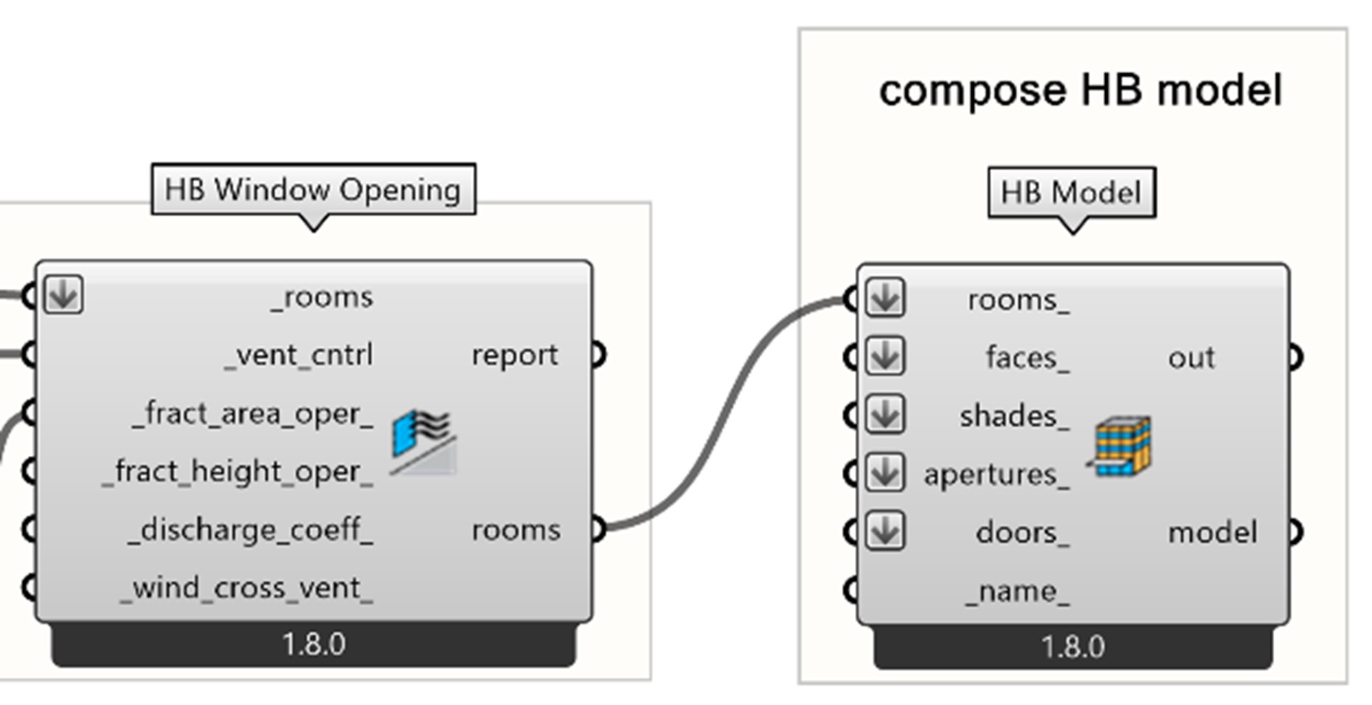
- Create a Model component.
- Connect the ‘rooms’ result from the HB Window Opening component to the corresponding input.
Important to note: You should connect only the ‘rooms’ result this time. If you connect any of the other inputs (e.g. some additional orphaned faces in the ‘faces_’ input), it will create an error in the energy simulation.
5. Visualize & Check the HB Model
Lastly, you need to visualize the HB Model to check that it is composed correctly. To quickly check the attributes that are assigned to each face:
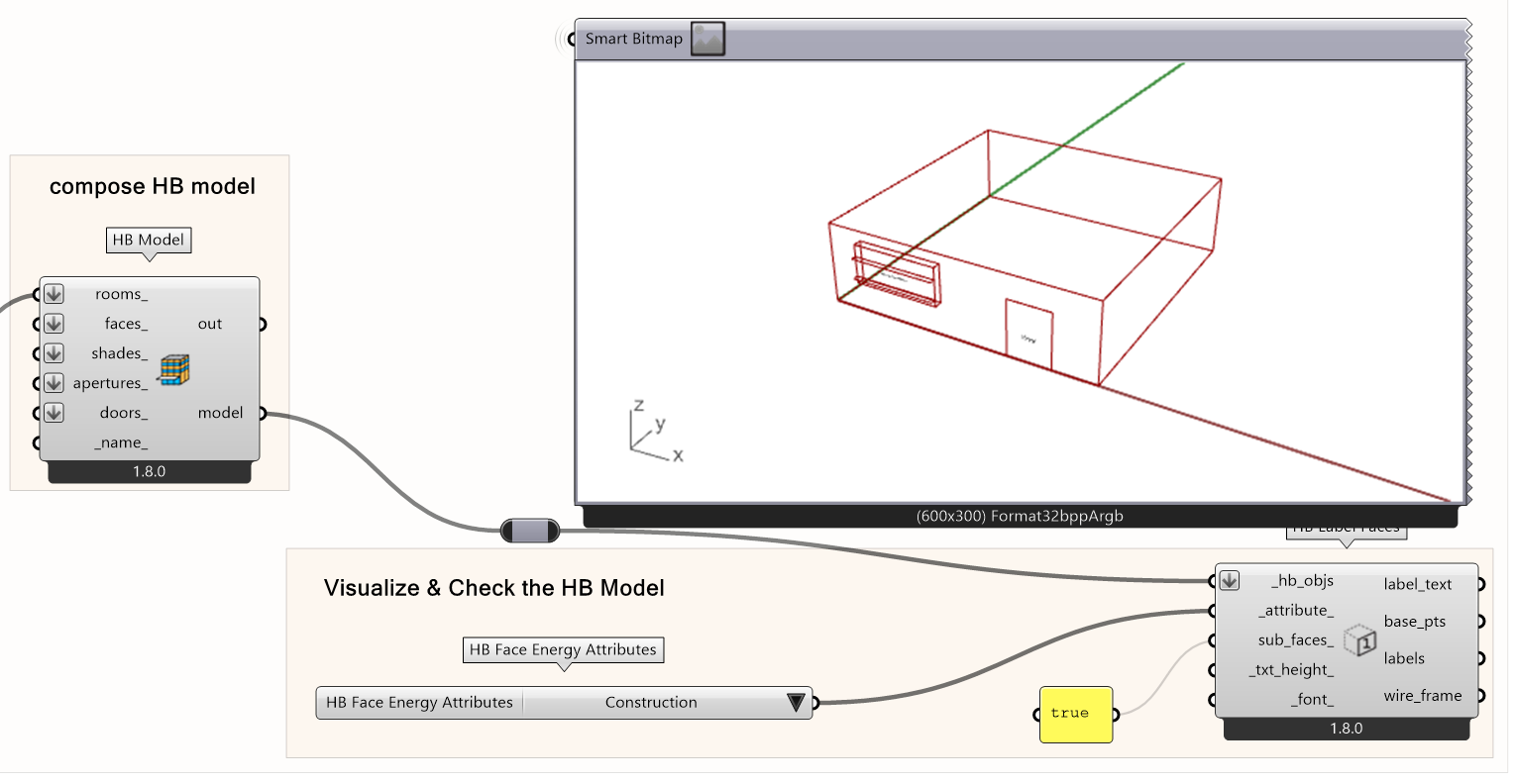
- Create a HB Label faces component.
- Connect the ‘model’ result from HB Model to the ‘_hb_objs’ input.
- Create a Face Energy Attributes component and select the attribute what you will show. For this tutorial, select the Construction attribute.
- Create a Panel and connect it to the ‘sub_faces_’ input. Write True if you want to label the window instead of the opaque surfaces.
Honeybee Energy Analysis with Open Studio 5/8
Create & Run the Open Studio simulationlink copied
The Open Studio simulation involves two steps for its creation before being able to run the energy simulation. You will need to import the weather data and set the simulation parameters.
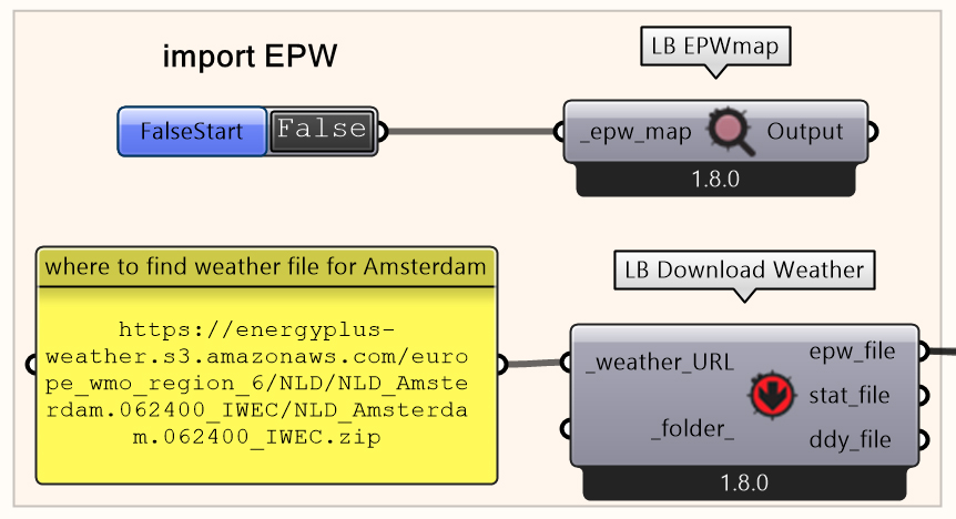
Import Weather Data
You can import and extract the respective EPW weather data by following the steps in Importing the EPW data section of the Importing weather files in Ladybug tutorial (only this section is needed for this tutorial and not the whole tutorial!).
Following these steps (and selecting the Amsterdam weather data in the EPW map), you should have the components as shown in the image. It is important to make sure that the EPW file we are using is of good quality and does not miss any data. See how you can check the quality of the EPW file in Importing weather files in Ladybug » Checking the quality of the EPW file.
Important to note: In case you are using the provided file, you have already imported the EPW weather data for the Point-in-Time simulation or the Annual Daylight simulation, and, therefore, you can use the same component.
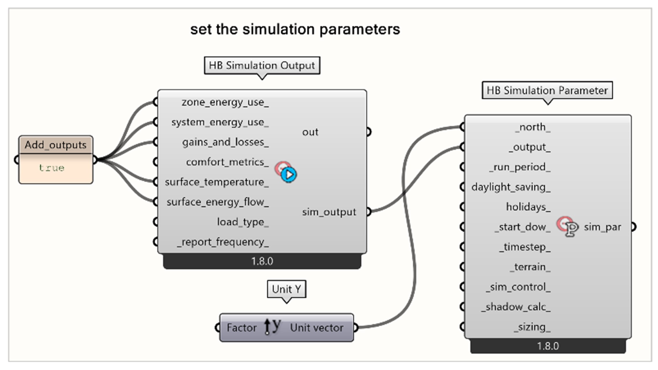
Set the Simulation Parameters
Next step to prepare the Energy simulation with Open Studio is to set the simulation parameters:
- Create an HB Simulation Output component.
HB – Energy » Simulate » HB Simulation Output
- Create a Panel component and set it to True. Connect it with all the ‘zone_energy_use_’, ‘hvac_energy_use_’, ‘gains_and_losses_’, ‘comfort_metrics_’, ‘surface_temperature_’, ‘surface_energy_flow_’ inputs.
Important to note: These inputs correspond to the values which are going to be calculated through the energy simulation. If you do not set an input to True, then the respective values are not going to be calculated, and you will get no result for them after the simulation.
- Create an HB Simulation Parameter component.
- Connect the ‘sim_output’ result of the HB Simulation Output component to the ‘_output_’ input.
- Define the north of the location. In this tutorial, the north vector will be set along the positive direction of the Y axis, facing the opposite direction of the aperture normal. Create a Unit Y vector component and connect the ‘unit vector’ result to the ‘north_’ input.
- In the ‘_run_period_’ you can define the analysis period for the simulation. You can follow a similar approach to the one described in Importing weather files in Ladybug tutorial » Specify time period in the WEA file. In this tutorial, we will run the simulation for the whole year (default option).
- By browsing your mouse over the rest of inputs, you can see which other parameters can be specified. You can find the respective auxiliary components for each of them on the Simulate subpanel.
Run the Energy Simulation
After preparing the parameters for the simulation, there are a few final steps to be able to run the Energy simulation. To run the simulation:
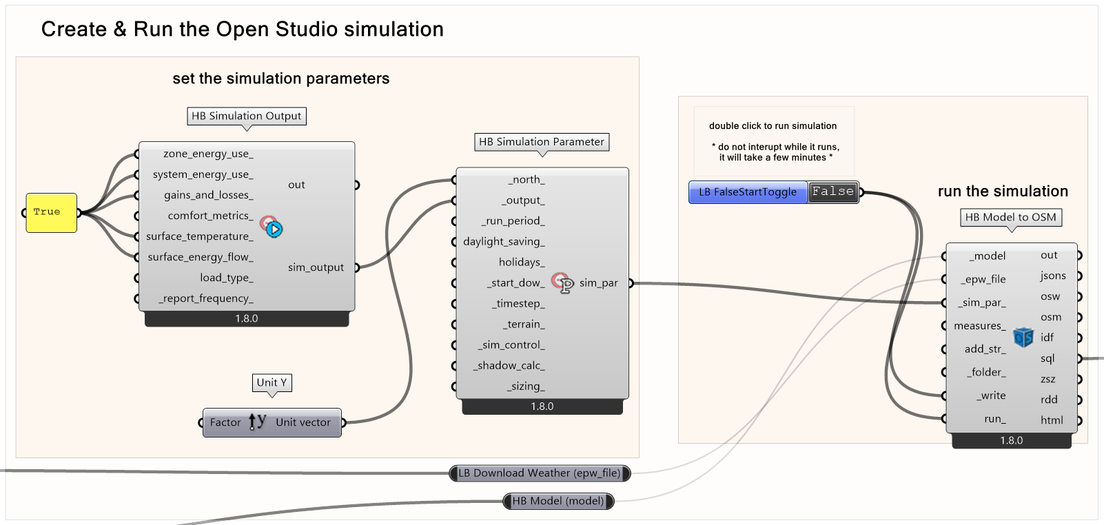
- Create an HB Model to OSM component.
- Connect the ‘model’ output of the HB Model component to the ‘_model’ input.
- Connect the ‘epw_file’ output of the LB Download Weather component to the ‘_epw_file’ input.
- Connect the ‘sim_par’ output of the HB Simulation Parameter component to the ‘_sim_par_’ input.
- Create a Boolean Toggle component and connect it to the ‘_write’ & ‘run_’ inputs of the HB Model to OSM component.
- Double-click the Boolean Toggle component to set it to ‘True’ and run the simulation.
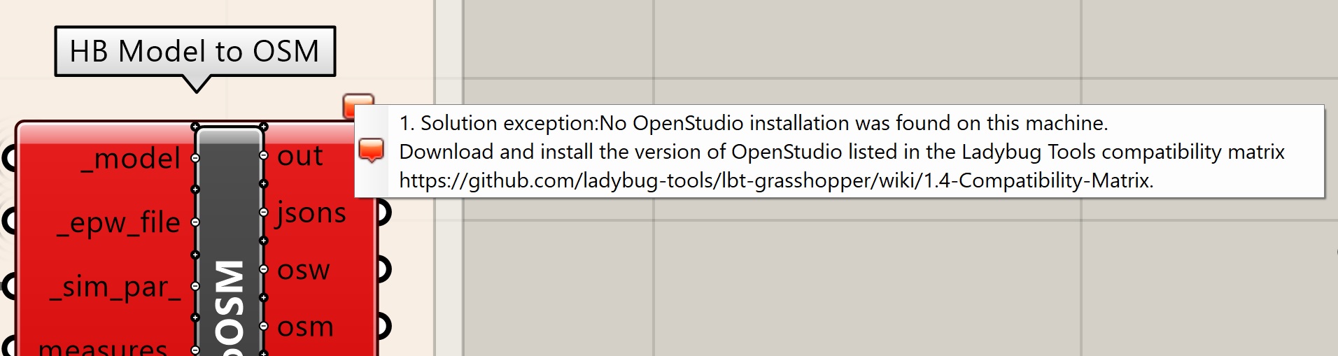
Possible Error: If the simulation does not run and you get this error then you can manually download the corresponding OpenStudio for your Ladybug version from github here and try again.
Honeybee Energy Analysis with Open Studio 6/8
Post-Processing the Resultslink copied
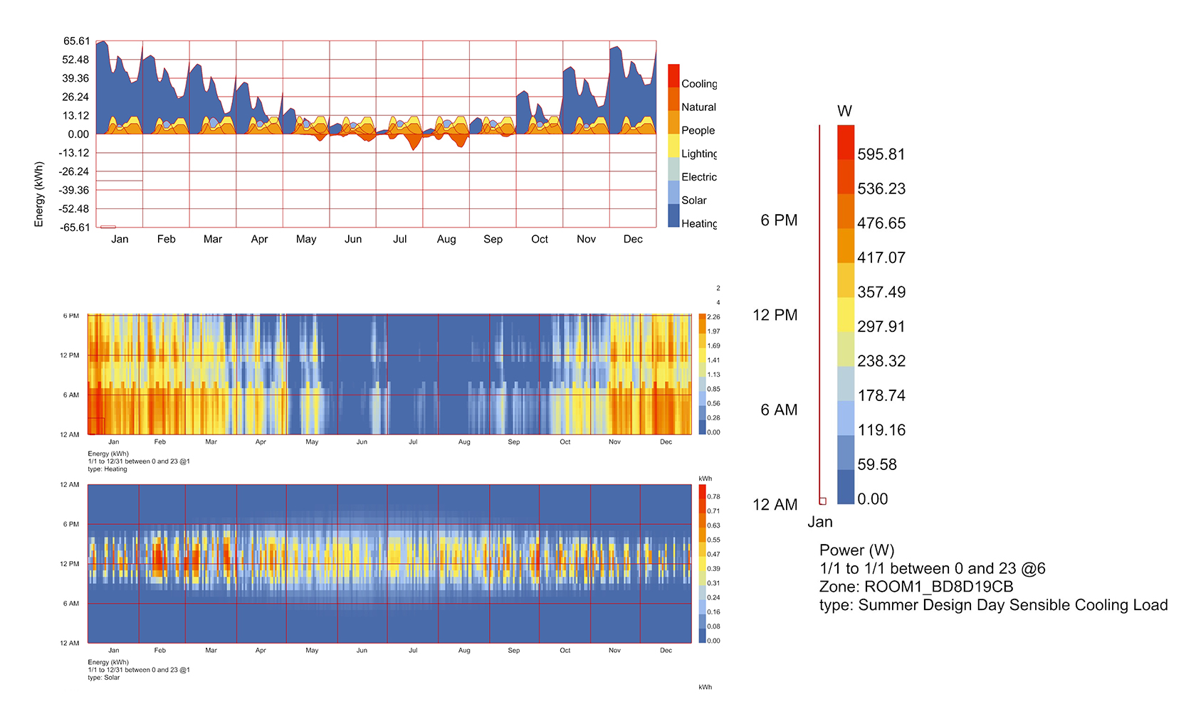
The final step of the Energy Analysis tutorial is to visualize and post-process the results of the Energy simulation. You will post-process the results regarding the Thermal Load Balance, Zone Sizing, Thermal Comfort and End Use Intensity.
Important to note: Some of the components may give ‘Empty Generic Data parameter’ as a result or appear to have a value of 0 although this does not seem realistic. The problem is either that the respective components are not added in the first phase (for our example, there is no HVAC system added in the HB model so the mechanical ventilation load will appear as 0) or that the respective calculation is not set to “True” on the HB Simulation Output component.
Thermal Load Balance
Here, the values regarding heating & cooling are going to be extracted, as well as the lighting & equipment energy needed in kWh, the heat loss / gain due to natural ventilation and the solar & internal heat gains.
Important to note:
A. The values regarding heating will always be positive and the values regarding cooling will be negative.
B. In this example, the heating & cooling loads refer to the total energy that needs to be added or removed from the room. In case there was a detailed HVAC system added, it would refer to the total electric energy needed for it.
To extract the Thermal Load Balance values:
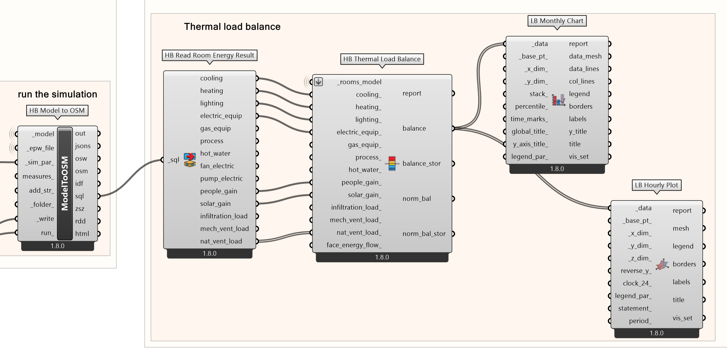
- Create an HB Read Room Energy Result component.
- Connect the ‘sql’ output of the HB Model to OSM component to the ‘_sql’ input.
- Create an HB Thermal Load Balance component.
- Connect the ‘model’ output of the HB Model component to the ‘_rooms_model’ input.
- Connect the ‘cooling’, ‘heating’, ‘lighting’, ‘electric_equip’, ‘people_gain’, ‘solar_gain’ and ‘nat_vent_load’ results of the HB Read Room Energy Result component to the respective inputs of the HB Thermal Load Balance component.
Important to note: Connect the HB Model component as it was created it in Compose the HB Model for the Energy Simulation.
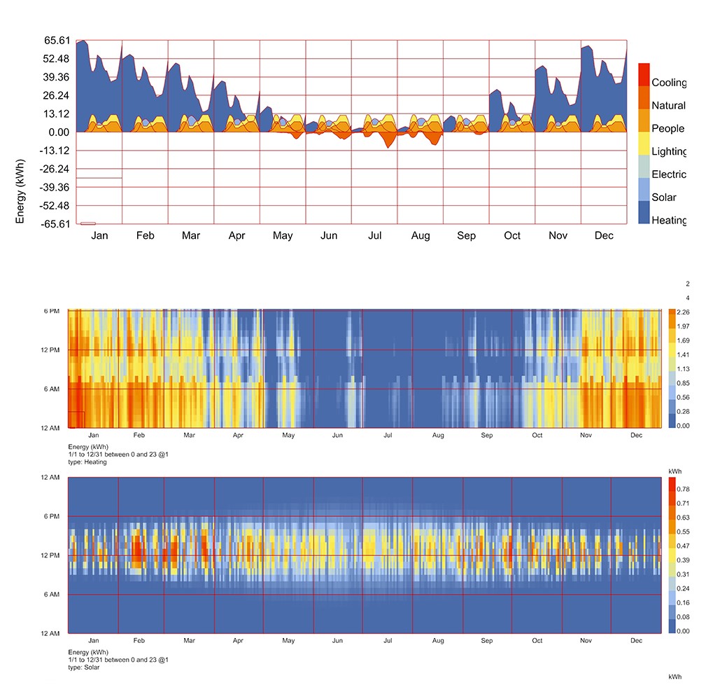
- Create a LB Monthly Chart component to visualize the data per hour or per month respectively. Connect the ‘balance’ or ‘norm_bal’(normalized by the floor area) result to the ‘_data’ input.
or
- You can see the resulting Map by clicking on the LB Hourly Plot or LB Monthly Chart component.
- The graph will appear on your Rhino scene.
Zone Sizing
To define the necessary equipment capacity, it is more common to use the heating & cooling loads calculated for the Heating & Cooling Design day, i.e. the days that refer to the worst case scenario in terms of the building’s energy needs.
To read the results regarding the Zone Sizing:
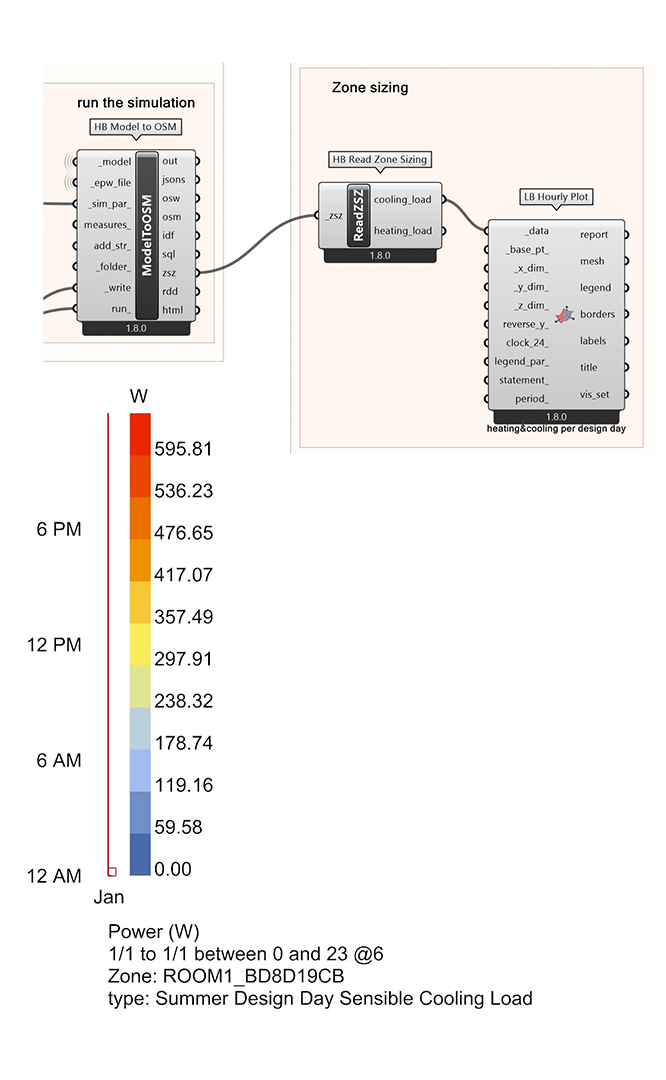
- Create an HB Read Zone Sizing component.
- Connect the ‘zsz’ output of the HB Model to OSM component to the ‘_zsz’ input.
- Create a LB Hourly Plot component and connect the ‘cooling_load’ or ‘heating_load’ result to the ‘_data’ input.
- You can see the resulting Map by clicking on the LB Hourly Plot component. The graph will appear on your Rhino scene.
- If you want to bake the graph:
Important to note: Since the values that we take this time refer only to the hours of one day, it only makes sense to use the LB Hourly Plot and not the LB Monthly Chart.
Thermal Comfort
The Thermal Comfort indicators refer to both the actual comfort (mean air temperature, mean radiant temperature – considering the radiant heat transfer from the human body – and mean relative humidity) and likely comfort (operative temperature – calculated taking into account all the aforementioned actual comfort indicators).
To visualize the simulation results for Thermal Comfort:
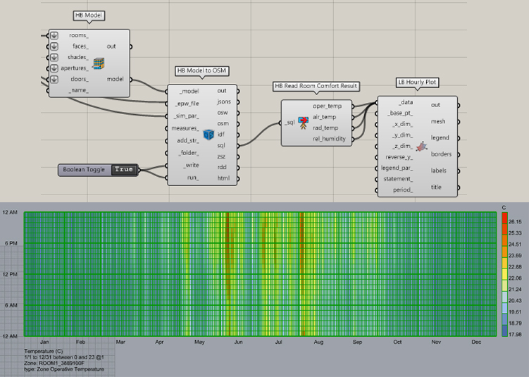
- Create an HB Read Room Comfort component.
- Connect the ‘sql’ output of the HB Model to OSM component to the ‘_sql’ input.
- Create a LB Hourly Plot or a LB Monthly Chart component to visualize the data per hour or per month respectively. Connect the data from all the different results to the ‘_data’ input.
- You can see the resulting Map by clicking on the LB Hourly Plot or LB Monthly Chart component. The graph will appear on your Rhino scene.
- If you want to bake the graph:
End Use Intensity
End Use Intensity is an indicator of the energy efficiency and is calculated as the sum of all the energy needs of the building divided by the gross floor area. The acceptable values differ based on the use of the building.
To view the End Use Intensity results of the simulation:
- Create an HB End Use Intensity component.
- Connect the ‘sql’ output of the HB Model to OSM component to the ‘_sql’ input.
- Create a Panel component and connect it to the ‘eui’ output. This will give you the total End Use Intensity Value.
Create 2 Panel components and connect it to the ‘eui_end_use’ and ‘end_uses’ output. These panels will give you the different end uses and the values that correspond to them.
Honeybee Energy Analysis with Open Studio 7/8
Conclusionlink copied
In this tutorial you learned how to set-up and run an Energy Analysis simulation using Honeybee and Open Studio. By following the steps explained in the tutorial you are now able to set construction sets and compose the program type along with assigning internal mass and setting natural ventilation parameters to compose the HB model for the Energy simulation. You have also learned hot to visualize the HB model to check that it is correctly composed. Moreover, you learned to create and run the Energy simulation with Open Studio and finally post-process its results regarding the Thermal Load Balance, Zone Sizing, Thermal Comfort and End Use Intensity.
Complete exercise file
Honeybee Energy Analysis with Open Studio 8/8
Useful Linkslink copied
Previous Tutorials
Follow-up Tutorials
Other Useful Links
OpenStudio for Ladybug download from github: https://github.com/NREL/OpenStudio/releases/tag/v3.7.0
Write your feedback.
Write your feedback on "Honeybee Energy Analysis with Open Studio"".
If you're providing a specific feedback to a part of the chapter, mention which part (text, image, or video) that you have specific feedback for."Thank your for your feedback.
Your feedback has been submitted successfully and is now awaiting review. We appreciate your input and will ensure it aligns with our guidelines before it’s published.