Workshop 4: Python Libraries
-
Intro
-
Libraries and Modules
-
NumPy (library)
-
Working with Image Data
-
Conclusion
Information
| Primary software used | Python |
| Software version | 1.0 |
| Course | Workshop 4: Python Libraries |
| Primary subject | Prototyping and Manufacturing |
| Secondary subject | Robot Programming |
| Last updated | March 3, 2026 |
| Keywords |
Responsible
| Teachers | |
| Faculty |
Workshop 4: Python Libraries 0/4
Workshop 4: Python Libraries
Learn to use python modules and external libraries to extend your program’s functionalities
This tutorial is published as part of a series of workshops for an interfaculty course from TU Delft Faculty of Architecture and the Built Environment to support learning in and outside the class with open learning material. The intent of the workshop series is to increase familiarity with programming language Python for research and scientific applications as part of the course Creative Robotics in Spatial Design.
You are free to go through the learning material at your own to get familiar with Python fundamentals.

Learning Objectives
- Differentiate between the utilities of a few popular Python libraries
- Develop functions based on the imported libraries
- Understand and analyze the underlying functions for image processing
Download Workshop Notebook (week 2, workshop 4)
The zip file contians the notebook and needed images/data to complete the workshop.
Previous Workshops
Below are the prior workshops that briefly covers a limited scope on the fundamentals of programming with Python.
Workshop 4: Python Libraries 1/4
Libraries and Moduleslink copied
In programming, a library is a collection of pre-written code: functions that developers can use to perform common tasks and solve problems without having to write code from scratch.
Libraries help to streamline development by providing reusable components, which can reduce code duplication and development time. They often include functions for specific domains or tasks, such as data manipulation, mathematical operations, or web development. Libraries can contain a collection of packages, which in turn are a collection of modules. A module is a single file containing Python code that defines functions, classes and variables.
In some IDE’s, like Google Colab, certain common libraries are already installed. However, you need to **import** libraries in Python to access their pre-written code, functions, and tools. And when using VS code (the IDE on your local computer), you will be required to install the libraries first before you can import (use) them.
Examples of Some Popular Libraries and Modules
A few popular libraries available to download:
- NumPy: Provides support for large, multi-dimensional arrays and matrices, along with a collection of mathematical functions to operate on these arrays.
- Pandas: Offers data structures like DataFrames and Series for data manipulation and analysis, making it easier to handle and analyze structured data.
- Matplotlib: A plotting library for creating static, animated, and interactive visualizations in Python. It is widely used for generating graphs and charts.
- SciPy: Builds on NumPy and provides additional functionality for scientific and technical computing, including modules for optimization, integration, interpolation, and more.
- PyTorch: An open-source library for machine learning and deep learning developed by Google, offering tools and frameworks for building and training neural networks.
Python Modules:
- os: Provides functions for interacting with the operating system, including file and directory operations. Functions like os.path.join() and os.listdir() are used for file management.
- math: Provides mathematical functions such as sqrt(), sin(), and log(). Useful for basic mathematical operations and calculations.
- datetime: Offers classes for manipulating dates and times, such as datetime, date, and time. Essential for handling date and time data.
- json: Provides methods for parsing JSON data and converting Python objects to JSON format. Useful for working with data interchange formats.
- csv: A module for reading and writing CSV (Comma-Separated Values) files, which provides functionality to handle tabular data in plain text format.
Library vs Module: For the extents and purposes of this workshop series, the distinction between these terms is not important. In the remainder of this chapter, these terms are used interchangably.
Importing Libraries
Unlike Grasshopper plug-ins, libraries are not automatically loaded in your script (otherwise, scripts would quickly become too heavy). Instead, they need to be imported manually.
We can choose to import the entire library, or to only import specific items. The code is pretty intuitive:
import mathor
from math import piIt is good practice to put all “import” statements at the top of the script. Note that, in addition to importing (loading) libraries in your script, some libraries also have to be installed as explained in the previous step.
Note: if you run modules/library functions without importing them first like ‘import math’, you will encounter an error. You only need to import a library (run “import math”) once; you do not need to import it for each code block
Below is an example of the library math:
import math

print(math.pi)

# output: 3.141592653589793
Once the module is imported, you can run any functions available from the module (see math documentation).
print(math.floor(3.82382))
print(math.ceil(1.0022352))
print(math.factorial(5))
print(math.radians(250))
print(math.sin(math.radians(15)))

# Output:
# 3
# 2
# 120
# 4.363323129985824
# 0.25881904510252074
Tip: it is good practice to have all import statements at the top of the script
Start with import module for maximum clarity.
If you prefer more direct access to a few specific functions, use from module import function.
For example:
from statistics import median, mean #you can now use these functions directly
from math import pi
"""
Notice that when we use the 'from statistics import median` syntax,
we do not need to refer to the module name statistics.median(my_list)
"""
my_list = [2,7,1,4,9,3]

print(pi)
print(median(my_list))
print(mean(my_list)*pi)

# Output:
# 3.141592653589793
# 3.5
# 13.613568165555769
In this example, there is no need to specify the module’s name anymore (‘math.pi’ for instance is now ‘pi’ only).
Installing Libraries (using Pip Package Manager)
Python comes pre-installed with the most commonly used and helpful libraries. However, sometimes you will need a special library that is not included in the pre-installation of Python. For this, you will use the `pip` command to install libraries directly from your notebook/terminal. If you are importing from within the Jupyter Notebook, use `%pip` as the command. And if you use the terminal, use `pip` as the command. Both should be followed by `install ‘library_name‘` to retreive it from the available libraries.
For example, to install a library that will help you plot graphs and view images as outputs in the notebook, you must install Matplotlib library.
%pip install matplotlib
# or directly in the terminal:
pip install matplotlib
You can find the pip install command on this repository: https://pypi.org/
Importing your Own Module
It is also possible that you create a module of your own. For example, you develop a set of functions that is critical for your workflow. Maybe it is functions to control your system, sensors, actuators, or something else that is not standard to any normal library available for download.
create a new .py file, and add all of your functions in that file, and save it in the same project directory as your main juputer/python file.
Your module should be in the same map/folder as the main file you are importing it from. Otherwise if you place them in sub-folders, you will have to look up a method to make it work for your project. If you update the functions in your module, restart your Jupyter notebook/kernel
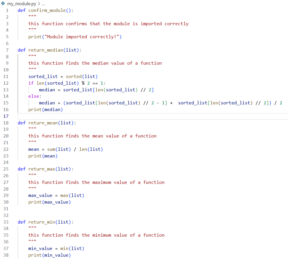
import my_module

my_module.confirm_module()
my_module.return_median([2,7,1,4,9,3])
my_module.return_mean([2,7,1,4,9,3])
my_module.return_max([2,7,1,4,9,3])
my_module.return_min([2,7,1,4,9,3])

# Output:
# Module imported correctly!
# 3.5
# 4.333333333333333
# 9
# 1Workshop 4: Python Libraries 2/4
NumPy (library)link copied
NumPy is a multi-dimensional array library for Python to store data in `n` dimensional arrays. NumPy is generally faster than list and allows for mathematical operations on arrays.
It is a fundamental package for scientific computing with Python and is widely used in data analysis, image manipulation, and machine learning. In short, NumPy arrays are faster, easily holds multi-dimensional arrays, and can manipulate the arrays using mathematical operations.
Its documentation can be found here.
We will cover just a few libraries in this workshop/tutorial mostly concerning with arrays and image data.
Array Data Type
Array data structures are similar to lists, but they are more efficient for numerical computations and data manipulation. Arrays can be of any dimension (1D, 2D, 3D, etc.) and can hold elements of the same data type.
We will work with array data structures using NumPy and in combination with other libraries which will be explained later. For now, Install all of these on your computer via your Jupyter Notebook:
# Install NumPy to work with arrays
%pip install numpy
# install openCV (cv2) to work with images
%pip install opencv-python
# isntall matplotlib to plot graphs and view images
%pip install matplotlib

import cv2  as cv # the OpenCV library
import numpy as np # NumPy library
import matplotlib.pyplot as plt # Matplotlib library
Compare these two operations below. A multiplication of two lists of the same length. This won’t work as expected because lists cannot be multiplied by each other.
a = [1, 2, 3]
b = [4, 5, 6]

x = a * b  # This will not work as expected, it will repeat the list
Arrays allow us to perform element-wise multiplication, where each corresponding pair of elements is multiplied together, resulting in a new array of the same shape.
arr_a = np.array([1,2,3]) # Convert list to NumPy array
arr_b = np.array([4,5,6])
arr_c = a * b

print(a)
print(b)
print(c)
print(f'the data type of the array items are: {c.dtype}')

# Output:
# [1 2 3]
# [4 5 6]
# [ 4 10 18]
# the data type of the array items are: int32
The values in the array are indicated as integers (int32). You can change the data type of the items in the array by using this following function.
# change the data type of the array items to float using .astype() method
arr_c_float = arr_c.astype(float)  # Use astype to convert array dtype
print(f'the data type of the array items are: {arr_c_float.dtype}')

# Output: the data type of the array items are: float64
Multi-Dimensional Arrays (1D, 2D, 3D)
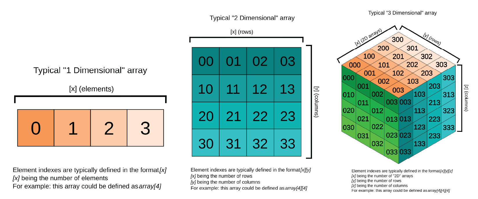
A multi-dimensional array is sort of like a list within a list, but it can be of any dimension.
For example, a 2D array is like a table with rows and columns, while a 3D array takes it a step further, creating a structure like a cube of data.
Example of different array dimensions:
# 2D array example:
array_2d = np.array([[1, 2, 3], [4, 5, 6]])

# 3D array example:
array_3d = np.array([[[1, 2], [3, 4]],      # first "layer"
                     [[5, 6], [7, 8]],      # second "layer"
                     [[9, 10], [11, 12]]])  # third "layer"

# count the number of dimensions:
print("Number of dimensions in 2D array:", array_2d.ndim)
print("Number of dimensions in 3D array:", array_3d.ndim)
# the shape of an array tells us how many elements it has in each dimension
print("Shape of 2D array:", array_2d.shape)
print("Shape of 3D array:", array_3d.shape)

# Output:
# Number of dimensions in 2D array: 2
# Number of dimensions in 3D array: 3
# Shape of 2D array: (2, 3)
# Shape of 3D array: (3, 2, 2)
Dive Deeper into NumPy
Working with NumPy arrays is a prerequisite for working with image data. Arrays are used to represent images in a way that computers can understand and manipulate. Fundamentally, arrays are just grids of numbers, and images can be represented as grids of pixel values.
You can learn the fundamentals of NumPy and working with array data structures by following online resources:
- NumPy Official Documentation: NumPy documentation — NumPy v2.3 Manual
- NumPy Tutorial by W3Schools: NumPy Tutorial
Workshop 4: Python Libraries 3/4
Working with Image Datalink copied
Image Data as NumPy Arrays
Image data are often represented as 2D or 3D NumPy arrays, where each element corresponds to a pixel value. To work with images, you will need to download additional modules. We will use OpenCV for that.
The idea is to start understanding what an image is for a computer and how we can ask a computer to ‘look’ at our image. For a computer, an image is nothing else than a succession of bits. These bits forms codes that tells the intensity of each of your Red, Green and Blue leds that are in your screen.
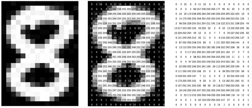
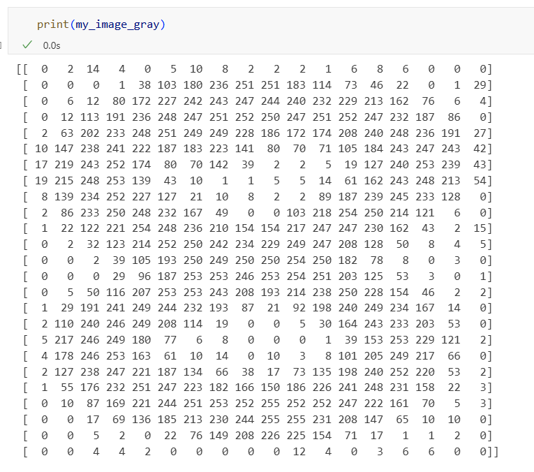
We can view the underlying NumPy array in grayscale:
– 0 and lower numbers represents black pixels
– as the values increases, it reaches towards white pixels
– 255 is the maximum value representing white pixels
Load your Image to Jupyter Notebook
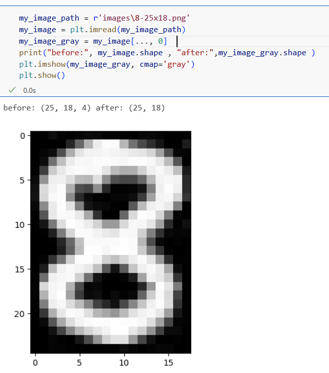
Set a variable name to the path of your image. For example, a relative path from the Jupyter notebook would be:
my_image_path = r'images\8-25x18.png'We can use Matplotlib to read the image as follows:
my_image = plt.imread(my_image_path)The image now has 4 channels (Red, Green, Blue, Alpha). We can isolate the array to only the first channel. We know our image is greyscale so it’s okay.
my_image_gray = my_image[..., 0] # takes all content from first channelDisplay the image using Matplotlib:
plt.imshow(my_image_gray, cmap='gray') #choose 'gray' color map 'cmap'
plt.show()
You will see the image displayed in the notebook.
Printing the image can show the array structure and each corresponding value of each pixel (255 being white and 0 being black). See image below.
So far we worked with single 2D arrays to represent images. The next sub-chapter explres some image manipulation using OpenCV library
RGB Image Arrays
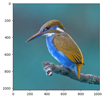
We update the file path to a new image in the directory and inspect the shape of the image.
image_1_path = r'images\kingfisher.jpg'
image_1 = cv.imread(image_1_path)

print("Sample image loaded successfully!")
print(f'the shape of the image is: {image_1.shape}

# Output:
# Sample image loaded successfully!
# the shape of the image is: (1024, 1024, 3)
View Image Using OpenCV (Pop-Up Window)
You can run the following script to display the image as a popup window. You will notice the image will appear on your computer in a separate window and can be closed by pressing any button on your keyboard.
#Display the image in a window
cv.imshow("Image Display", image_1)

# waitKey(0) waits indefinitely until any key is pressed
cv.waitKey(0)

# closes all the opened windows
cv.destroyAllWindows()
Notice that the image looks normal in terms of color representation.
However, if you display it on Matplotlib, the colors are mixed up:
plt.imshow(image_1)By default, OpenCV uses BGR default channel order for color images.
Convert Images to Grayscale and RGB
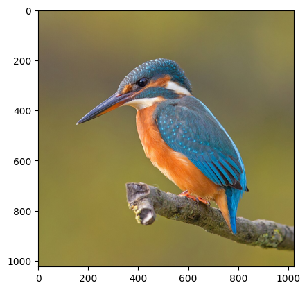
To convert the image to RGB values, you can use a function from OpenCV to make it simple to convert in the future:
image_1_path = r'images\kingfisher.jpg'
image_1 = cv.imread(image_1_path)
# convert from BGR to RGB color space
image_1_rgb = cv.cvtColor(image_1, cv.COLOR_BGR2RGB)

plt.imshow(image_1_rgb)

Converting to grayscale will require a change in the cvtColor function as follows:
image_1_path = r'images\kingfisher.jpg'
image_1 = cv.imread(image_1_path)
image_1_gray = cv.cvtColor(image_1, cv.COLOR_BGR2GRAY)
plt.imshow(image_1_gray, cmap='gray')
Image Transformation
Image transformation using python allows you to manipulate images in various ways, such as resizing, rotating, cropping, and applying filters. We will use OpenCV library for this purpose, but there are other libraries like PIL (Pillow) that can also be used for image manipulation.
You can use various transformation to your image arrays to emphasize important details in the image.
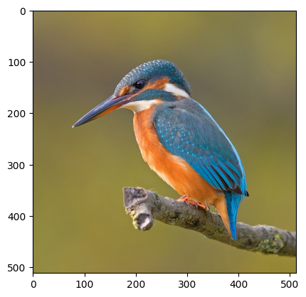
Image Resizing
Resizing an image using the .resize function.
image_1_resized = cv.resize(image_1_rgb, (512, 512))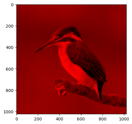
Manipulate RGB Channels
You can isolate specific color channels by indexing the array. I.e., to turn all the values in two of the three channels to 0. Note, you need to create a copy of the array to avoid modifying the original data.
# using array indexing
image_1_copy_1 = image_1_rgb.copy()
# image_1_copy_1[:,:,0] = 0
image_1_copy_1[:,:,1] = 0
image_1_copy_1[:,:,2] = 0

plt.imshow(image_1_copy_1)
print(image_1_copy_1.shape)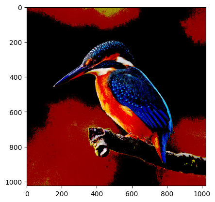
Apply a Mask
You can apply a mask to an image to highlight specific pixels. In this example, a boolean mask is created to “switch off” pixels with a value smaller than 100 in all channels.
# 1. Create a copy of the image to modify
image_masked_boolean = np.copy(image_1_rgb)

# 2. Create the boolean mask.
# This finds all pixel values NOT meeting the condition.
# The mask will be 'True' for every value less than or equal to 140.
mask = image_masked_boolean <= 140

# 3. Use the mask to set all 'True' elements to 0
# NumPy automatically selects only the pixels where the mask is True
# and sets those pixel values to 0 (black).
image_masked_boolean[mask] = 0

# The result is identical to the np.where method
plt.imshow(image_masked_boolean)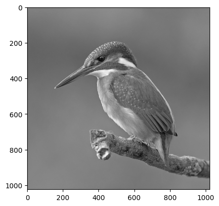
Convert to Grayscale Image Array
Using OpenCV function to convert to grayscale
image_1_gray = cv.cvtColor(np.copy(image_1_rgb), cv.COLOR_RGB2GRAY)
plt.imshow(image_1_gray, cmap='gray')
# Use color map 'cmap='gray' grayscale
images correctly
print(image_1_gray.shape)
Thresholding with NumPy
You can use NumPy to apply a threshold to a grayscale image. This will convert the image to a binary image where pixels above a certain value are set to white (255) and those below are set to black (0).
What is thresholding? Thresholding is a technique used in image processing to create binary images from grayscale images (see Wikipedia, OpenCV).
# Create a copy of the grayscale image to modify
image_thresholded = np.copy(image_1_gray)

# Apply thresholding
# Set pixels < 144 to black
image_thresholded[image_thresholded < 144] = 0
# Set pixels >= 144 to white
image_thresholded[image_thresholded >= 144] = 255

plt.imshow(image_thresholded, cmap='gray')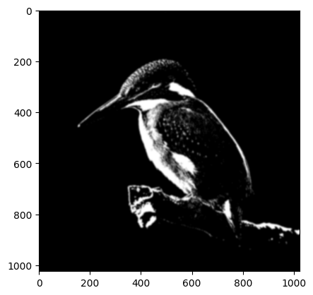
Gaussian Blur
You can apply a Gaussian blur to an image using OpenCV’s `GaussianBlur` function using the clipped image from the previous step.
# a simple blur effect using built-in OpenCV function
# (15, 15) is the kernel size, it must be odd and positive
image_blurred = cv.GaussianBlur(image_thresholded, (15, 15), 0)
plt.imshow(image_blurred, cmap='gray')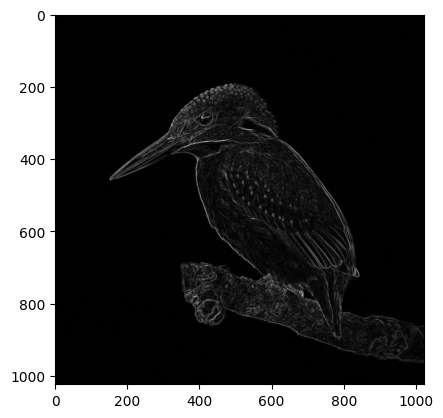
Edge Detection: Sobel Operator
Edge detection is a technique used to identify the boundaries within images. Here we use one of the techniques available in OpenCV, the Sobel operator.
# a simple edge detection effect using sobel operator from openCV

# Sobel in x direction
image_sobel_x = cv.Sobel(np.copy(image_1_gray), cv.CV_64F, 1, 0, ksize=5)
# Sobel in y direction
image_sobel_y = cv.Sobel(np.copy(image_1_gray), cv.CV_64F, 0, 1, ksize=5)
# Combine both directions
image_sobel = cv.magnitude(image_sobel_x, image_sobel_y)

plt.imshow(image_sobel, cmap='gray')
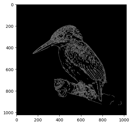
Edge Detection: Canny Edge
You can apply a Canny Edge Detection using OpenCV’s `Canny` function. It is good for detecting wide range of edges in images.
# you can adjust the two threshold values to get different results
image_edges = cv.Canny(np.copy(image_1_gray), 255, 255)

plt.imshow(image_edges, cmap='gray')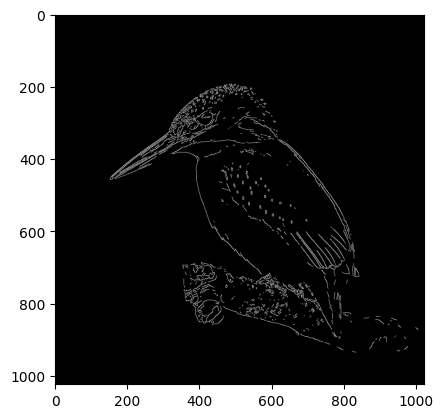
Combine Filters
You can combine multiple filters to create interesting effects. For example, applying a Gaussian blur followed by edge detection.
# first, blur filter
image_1_gray_blurred = cv.GaussianBlur(np.copy(image_1_gray), (5, 5), 0)

# Then, edge detection
canny_edges = cv.Canny(np.copy(image_1_gray_blurred), 125, 150)

plt.imshow(canny_edges, cmap='gray')
Image Processing Resources
Image processing is a vast field with many techniques and applications. Below are some nice resources to understand the theory behind filters and read more about the documentation on the techniques used here with OpenCV. Image processing is a nice prerequisite if you wish to learn about computer vision and machine learning.
- Nice summary of the theory behind blur filter: https://www.youtube.com/watch?v=C_zFhWdM4ic&ab_channel=Computerphile
-
OpenCV examples: https://docs.opencv.org/4.x/d4/d13/tutorial_py_filtering.html
- Computer vision crash course: https://youtu.be/-4E2-0sxVUM?feature=shared
- Additional exercises using OpenCV:
Workshop 4: Python Libraries 4/4
Conclusionlink copied
In this workshop/tutorial, we covered some popular Python libraries and modules, how to import them, and how to use them for basic image processing tasks. We explored NumPy for array manipulation, OpenCV for image processing, and Matplotlib for visualization. There are way many more libraries that you will encounter during your learning journey, some of which you might be using more often than others depending on what your end goal is.
You should now know how to:
- import a module/library
- install external libraries
- Use functions specific to the libraries
Previous Workshops
Follow-Up Workshop
Write your feedback.
Write your feedback on "Workshop 4: Python Libraries"".
If you're providing a specific feedback to a part of the chapter, mention which part (text, image, or video) that you have specific feedback for."Thank your for your feedback.
Your feedback has been submitted successfully and is now awaiting review. We appreciate your input and will ensure it aligns with our guidelines before it’s published.