Spectral Clustering
-
Intro
-
Overview
-
Training a Model
-
Applying a Transformation
-
Conclusions
Information
| Primary software used | Jupyter Notebook |
| Course | Spectral Clustering |
| Primary subject | AI & ML |
| Secondary subject | Machine Learning |
| Level | Intermediate |
| Last updated | November 27, 2024 |
| Keywords |
Responsible
| Teachers | |
| Faculty |
Spectral Clustering 0/4
Spectral Clustering
For this tutorial you need to have installed Python, Jupyter notebooks, and some common libraries including Scikit Learn. Please see the following tutorial for more information.
Download the Jupyter notebook here to follow along with the tutorial.
Spectral Clustering 1/4
Overviewlink copied

Spectral Clustering uses the eigenvalues of the similarity matrix of data to reduce their dimensionality and thus cluster them in a low dimensional manifold. It relates to graph theory and the concept of identifying groups of nodes based on the edges connecting them. Spectral Clustering is useful when the structure of a cluster is highly non-convex, or when a measure of the center and spread of a cluster does not describe a complete cluster. This happens, for example, when clusters are nested circles on a 2D plane.
Spectral Clustering 2/4
Training a Modellink copied
Dataset
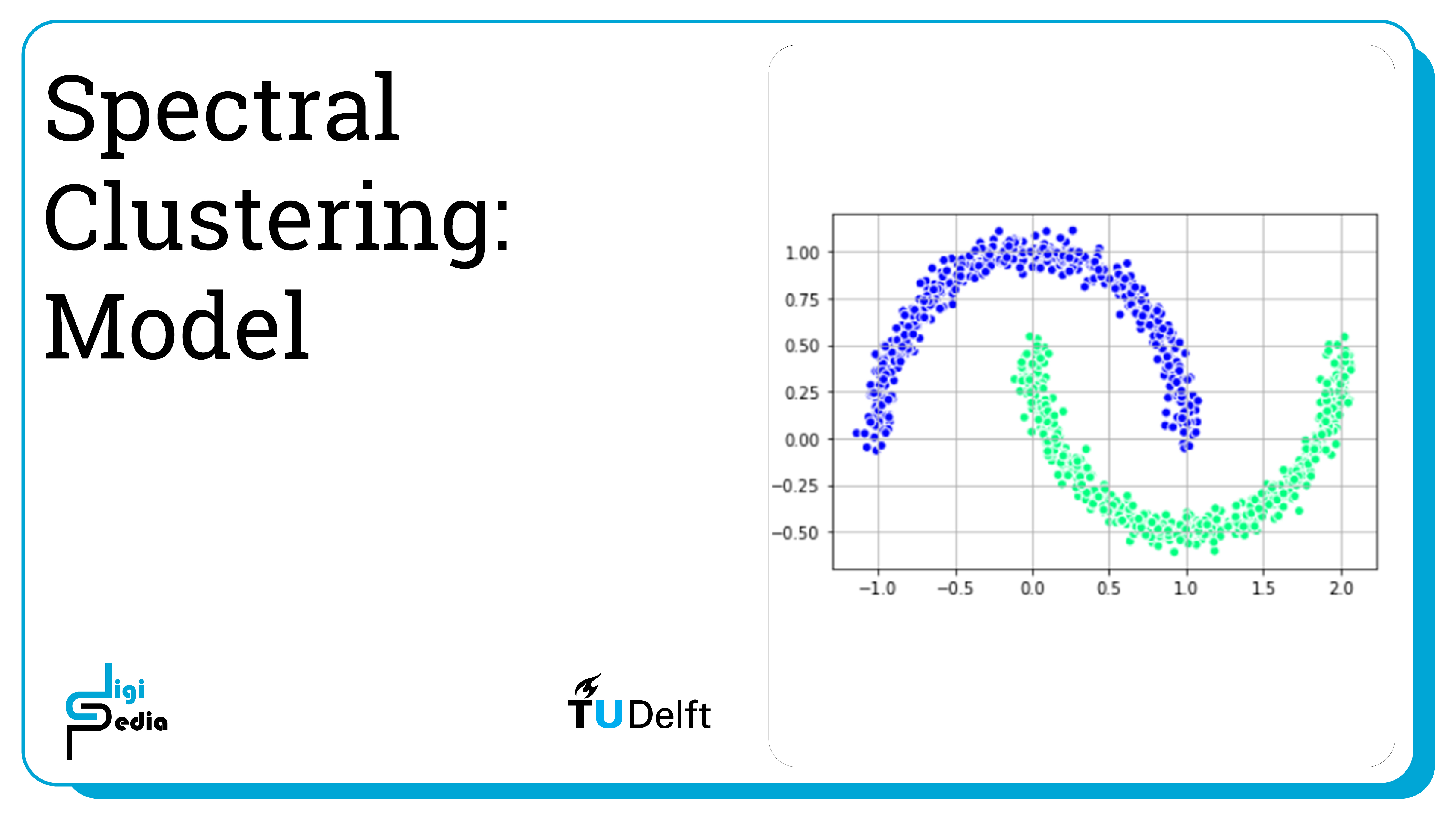
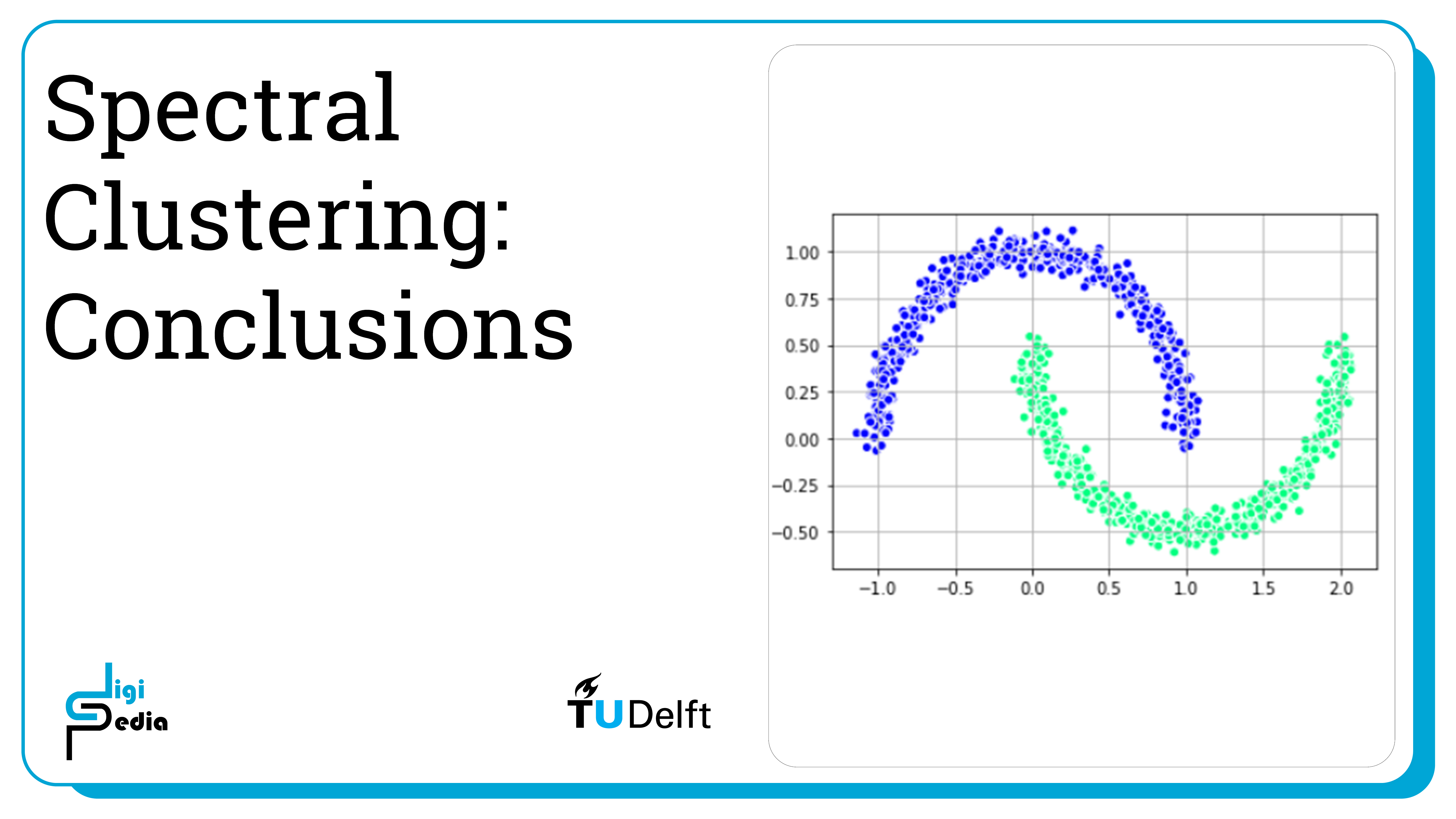
For this notebook, we will use a generated dataset in the shape of two intersecting half moons. We can generate and visualize the dataset below.
from sklearn.datasets import make_moons
X, y = make_moons(n_samples=1000, noise=0.05)

import matplotlib.pyplot as plt
# plot
plt.scatter(
   X[:, 0], X[:, 1],
   c='white', marker='o',
   edgecolor='black', s=50
)
plt.show()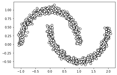
K-Means
We saw in the previous notebook that K-Means works well for data sets that have a cluster structure that is spherical like the example data set used in that notebook. Now, let’s take a look at a moon-shaped dataset. K-means cannot successfully cluster data in these configurations (even though visually we can see two clusters) because it uses a distance matrix to group points to a centroid. Below we will see what happens when we try to apply K-Means.
from sklearn.cluster import KMeans

clusters = 2

km = KMeans(
    n_clusters=clusters, init='random',
    n_init=16, max_iter=300,
    tol=1e-04, random_state=0
)
y_km = km.fit_predict(X)
# plot the 3 clusters
colors = ['lightgreen', 'orange', 'lightblue', 'lightcoral', 'gold', 'plum', 'midnightblue', ' indigo', 'sandybrown']
markers = ['s', 'H', 'v', 'p', '^', 'o', 'X', 'd', 'P' ]
for i in range(clusters):
plt.scatter(
X[y_km == i, 0], X[y_km == i, 1],
s=50, c=colors[i],
marker=markers[i], edgecolor='black',
label='cluster ' + str(i)
)
# plot the centroids
plt.scatter(
km.cluster_centers_[:, 0], km.cluster_centers_[:, 1],
s=250, marker='*',
c='red', edgecolor='black',
label='centroids'
)
plt.legend(scatterpoints=1)
plt.grid()
plt.show()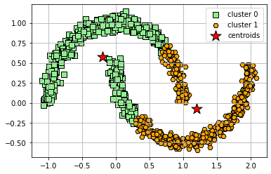
Since we know that k-means does not work, we need another clustering option. This is where spectral clustering comes in. For this example, we will use the generated dataset with the two intersecting moon shapes we just tried to cluster above.
Train a classifier using the SpectralClustering method and visualize it with the half moon dataset.
from sklearn.cluster import SpectralClustering
from sklearn.preprocessing import StandardScaler, normalize
from sklearn.decomposition import PCA
import pandas as pd
# Building the clustering model
spectral_model_rbf_2 = SpectralClustering(n_clusters = 2, affinity ='nearest_neighbors')
# Training the model and Storing the predicted cluster labels
labels_rbf_2 = spectral_model_rbf_2.fit_predict(X)
plt.scatter(X[:, 0], X[:, 1],
c = labels_rbf_2, edgecolor='white', cmap =plt.cm.winter)
plt.grid()
plt.show()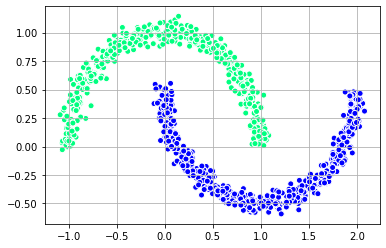
Spectral Clustering 3/4
Applying a Transformationlink copied
Dataset
It is also possible to find other methods to change the dimensionality of the data. First, let’s take a look at a dataset that consists of an inner circle and an outer ring. Spectral Clustering is able to classify the data.
import matplotlib.pyplot as plt
from sklearn.datasets import make_circles

#Generate data set
X_1, y_1 = make_circles(n_samples=(300, 100), shuffle=True, noise=0.05, factor=0.1, random_state=3)

# Plot data set
plt.scatter(
   X_1[:, 0], X_1[:, 1],
   c='black', marker='o',
   edgecolor='white', s=50
)
plt.grid()
plt.show()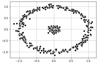
Clustering with Spectral Clustering
We can first see the clusters with spectral clustering.
# Building the clustering model
spectral_model_nn = SpectralClustering(n_clusters = 2, affinity ='nearest_neighbors')

# Training the model and Storing the predicted cluster labels
labels_nn = spectral_model_nn.fit_predict(X_1)

plt.scatter(X_1[:, 0], X_1[:, 1],
           c = labels_nn, edgecolor='white', cmap =plt.cm.winter)
plt.grid()
plt.show()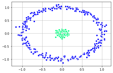
Clustering by Transforming the Data
Alternatively, we can apply a transformation to the data set ourselves to reduce the dimensionality. For the dataset above, we can find the distance to the center (0,0) in this case. This transforms the dataset to one-dimensional space and the data becomes linearly separable. We can then apply K-Means to get the clusters.
import numpy as np
import copy

#Distance to 0,0
X_1_np = np.array(X_1) #points in dataset
dist = (X_1_np[:, 0] ** 2 + X_1_np[:, 1] ** 2) ** 0.5 #get distance to zero
dist_coord = np.array(list(zip(dist, np.zeros(dist.shape))))

#Plot
plt.scatter(dist_coord[:,0], dist_coord[:,1],
           c = 'black', edgecolor='white', cmap =plt.cm.winter)
plt.grid()
plt.show()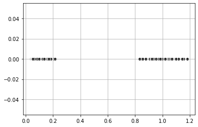
from sklearn.cluster import KMeans

#K-Means with Visualization
km = KMeans(
    n_clusters=2, init='random',
    n_init=10, max_iter=300,
    tol=1e-04, random_state=0
    )

y_km = km.fit_predict(dist_coord)


plt.scatter(dist_coord[y_km == 0,0], dist_coord[y_km == 0, 1],
           label = 'cluster 1', edgecolor='white', cmap =plt.cm.winter)
plt.scatter(dist_coord[y_km == 1,0], dist_coord[y_km == 1, 1],
           label = 'cluster 2', edgecolor='white', cmap =plt.cm.winter)
plt.legend(scatterpoints=1)
plt.grid()
plt.show()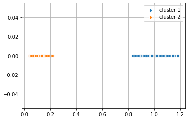
#Apply labels determined by K-Means back to the origional data set

plt.scatter(X_1[y_km == 0,0], X_1[y_km == 0, 1],
           label = 'cluster 1', edgecolor='white', cmap =plt.cm.winter)
plt.scatter(X_1[y_km == 1,0], X_1[y_km == 1, 1],
           label = 'cluster 2', edgecolor='white', cmap =plt.cm.winter)
plt.legend(scatterpoints=1)
plt.grid()
plt.show()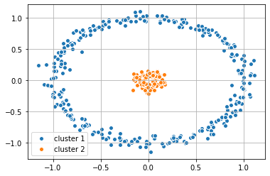
Spectral Clustering 4/4
Conclusionslink copied
- Spectral Clustering uses the eigenvalues of the similarity matrix of data to reduce the data’s dimensionality and then clusters it in fewer dimensions
- It draws inspiration from graph theory and the concept of identifying groups of nodes based on the edges connecting them
- Spectral Clustering is useful when the structure of a cluster is highly non-convex or when a measure of the center and spread of a cluster does not describe a complete cluster
- It is possible to use a similar process without implementing spectral clustering by transforming data to a lower dimension and then applying K-Means or Gaussian Mixtures on the linearly separable data
Write your feedback.
Write your feedback on "Spectral Clustering"".
If you're providing a specific feedback to a part of the chapter, mention which part (text, image, or video) that you have specific feedback for."Thank your for your feedback.
Your feedback has been submitted successfully and is now awaiting review. We appreciate your input and will ensure it aligns with our guidelines before it’s published.
