Random Forest / Decision Trees
-
Intro
-
Overview
-
Decision Trees
-
Random Forest
-
Conclusions
Information
| Primary software used | Jupyter Notebook |
| Course | Computational Intelligence for Integrated Design |
| Primary subject | AI & ML |
| Secondary subject | Machine Learning |
| Level | Intermediate |
| Last updated | February 25, 2025 |
| Keywords |
Responsible
| Teachers | |
| Faculty |
Random Forest / Decision Trees 0/4
Random Forest / Decision Trees
Random forest is an ensemble learning technique that combines the predictions of numerous decision trees, each trained on different subsets of the data, to enhance overall model performance. By averaging the predictions (in regression) or taking the majority vote (in classification), random forest reduces the risk of overfitting and improves generalization to new data. Additionally, it provides insights into feature importance, making it a powerful tool for both prediction and understanding the underlying data relationships.
For this tutorial you need to have installed Python, Jupyter notebooks, and some common libraries including Scikit Learn. Please see the following tutorial for more information.
Download the Jupyter Notebook below
Random Forest / Decision Trees 1/4
Overviewlink copied
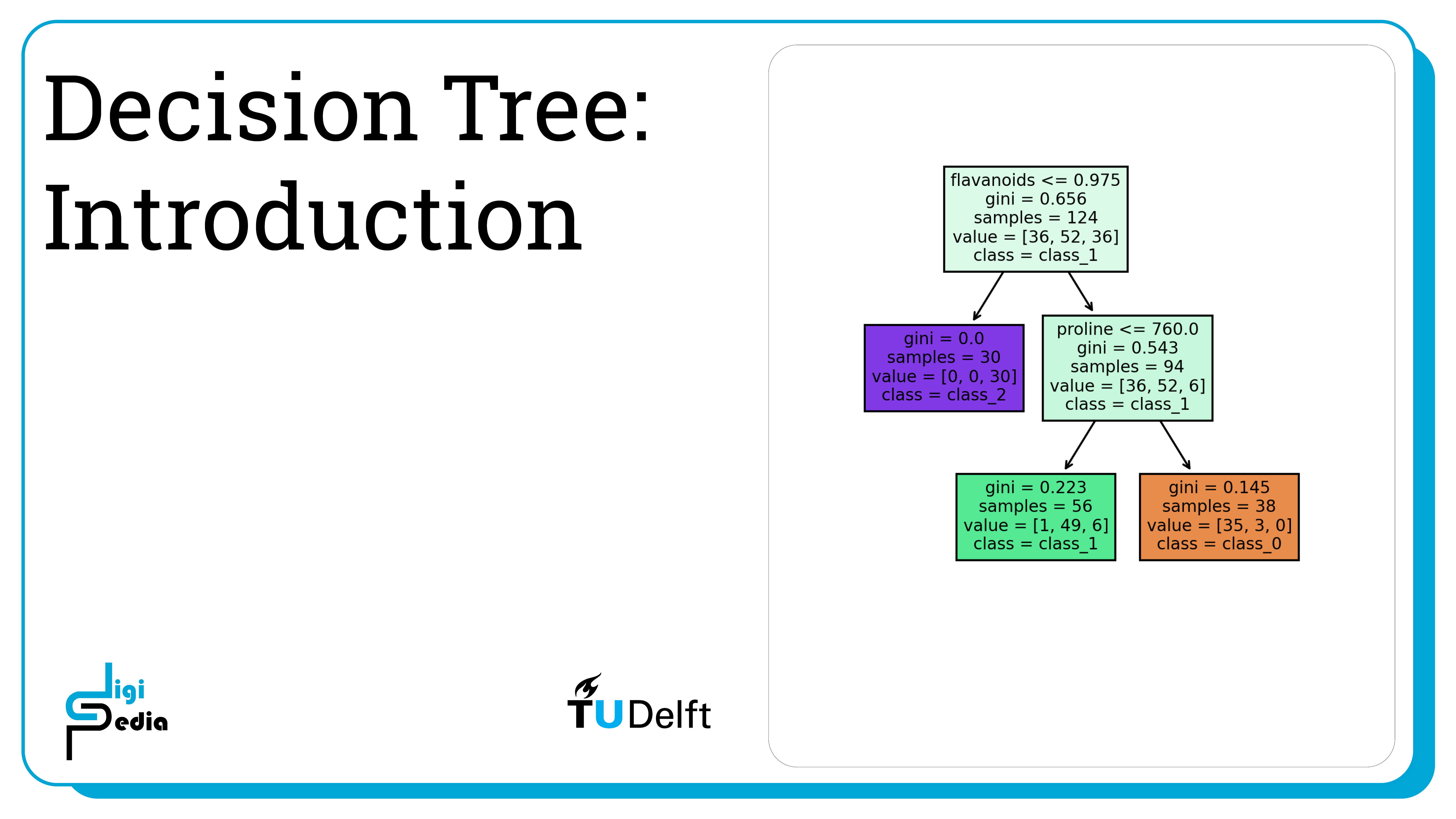
Decision Trees can provide an efficient classification option when data cannot be separated linearly. The most commonly used decision tree classifier splits the dataset into hyperrectangles with sides parallel to the axes. Decision trees start with the root node which contains the entire data set. The root node then splits into two descendant nodes. The splits continue until a leaf node is determined which contains data of only one class. At each split, the classifier creates nodes that are more homogeneous in regards to the class when compared to the ancestor’s subset of the datapoints. At each node, the classifier measures node impurity and splits the node so that the impurity of the descendant nodes is optimally decreased. Two common measures of impurity are Gini impurity and Entropy impurity.
Gini impurity is equal to one minus the sum of the probability of the datapoint belonging to each class squared.
equation
The maximum value is when the probability of the sample being assigned to all classes is the same. In a classification problem with three classes, this is approximately 0.667. The minimum value is when the node contains only one class and the value becomes 0.
Entropy impurity is determined by the entropy equation from Shannon’s Information Theory.
equation
The maximum value is also when the probability of the sample being assigned to all classes is the same. The minimum value is when the node contains only one class and the value becomes 0.
Entropy impurity takes more computational power to compute so Gini impurity is more widely used.
In addition to determining the purity of each node, the classifier needs criteria for stopping. One option is to stop when the node is pure (all datapoints in the node belong to one class). Another option is to stop when a node contains a small enough subset of data regardless of if the node is pure. By default, the decision tree classifier in SciKit Learn stops when the node is pure. Additionally, it is possible to set the max_depth parameter allows control over the size of the tree to prevent overfitting.
Like with all classifiers, data trees can overfit to the data when the tree is too large. When this is the case, the tree learns the details of a training set and these details cannot be generalized to new datapoints. The most common strategy is to grow the tree to a large size and then prune nodes.
Random Forest / Decision Trees 2/4
Decision Treeslink copied
# Load libraries
from sklearn.tree import DecisionTreeClassifier # Import Decision Tree Classifier
from sklearn.model_selection import train_test_split # Import train_test_split function
from sklearn import metrics # Import scikit-learn metrics module for accuracy calculation

# Import scikit-learn dataset library
from sklearn import datasets

# Load dataset
wine = datasets.load_wine()
It can be helpful to print certain characteristics of the dataset.
# print the names of the features
print(wine.feature_names)

['alcohol', 'malic_acid', 'ash', 'alcalinity_of_ash', 'magnesium', 'total_phenols', 'flavanoids', 'nonflavanoid_phenols', 'proanthocyanins', 'color_intensity', 'hue', 'od280/od315_of_diluted_wines', 'proline']

# print the label species(class_0, class_1, class_2)
print(wine.target_names)

['class_0' 'class_1' 'class_2']

Train a classifier using a 70/30 train test split and print the accuracy.

# Split dataset into training set and test set
X_train, X_test, y_train, y_test = train_test_split(wine.data, wine.target, test_size=0.3, random_state=1) # 70% training and 30% test
As discussed, it is possible to set the max_depth parameter allows control over the size of the tree to prevent overfitting. You can see the impact of overfitting by plotting the relative misclassification cost against the number of terminal nodes. The misclassification rate is calculated by taking the number of incorrect predictions and dividing these by the total number of predictions. The plot below shows that 9 terminal nodes is optimal because it allows for a low misclassification rate but the tree isn’t too large for overfitting to be a problem.
Max Depth
# change this to max depth
from matplotlib import pyplot as plt
terminal_nodes = []
accuracy = []

for i in range(1, 6):
# Create Decision Tree classifer object
clf = DecisionTreeClassifier(max_depth=i)
# Train Decision Tree Classifer
clf = clf.fit(X_train,y_train)
# Predict the response for test dataset append accuracy for plotting
y_pred = clf.predict(X_test)
terminal_nodes.append(clf.tree_.node_count)
accuracy.append(1 - metrics.accuracy_score(y_test, y_pred))

plt.plot(terminal_nodes, accuracy, '-o')
plt.title('Misclassification vs Terminal Nodes')
plt.xlabel('Number of Terminal Nodes')
plt.ylabel('Relative Misclassification Cost')
plt.show()
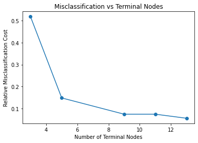
TASK 1: When training the model, the hyperparameter for the SciKit function is the maximum depth, not the number of terminal nodes. Now plot the Relative Misclassification Cost against the Maximum Depth to decide which max_depth value to use for the classifier.
TASK 2: The classifier below is trained with a max_depth value of 2. Based on the plot above, what value is more accurate? Update the max_depth value below.
Train Decision Tree Classifier
# Create Decision Tree classifer object
clf = DecisionTreeClassifier(max_depth = 2)
# Train Decision Tree Classifer
clf = clf.fit(X_train,y_train)
# Predict the response for test dataset
y_pred = clf.predict(X_test)
print(y_pred)
The output is:
[2 1 0 1 0 2 1 0 2 1 0 1 1 0 1 1 1 0 1 0 0 1 1 0 0 2 0 0 0 2 1 1 1 0 1 1 1 1 1 0 0 2 2 1 0 0 1 0 0 0 1 2 2 0]
# Number of Terminal Nodes
print("Terminal Node Count:", clf.tree_.node_count)
# Model Accuracy, how often is the classifier correct?
print("Accuracy:",metrics.accuracy_score(y_test, y_pred))

# Which classes are commonly misclassified?
print('Confusion Matrix')
print(metrics.confusion_matrix(y_test, y_pred, labels=None))
The output is:
Terminal Node Count: 5
Accuracy: 0.8518518518518519
Confusion Matrix
[[21 2 0]
[ 1 17 1]
[ 0 4 8]]
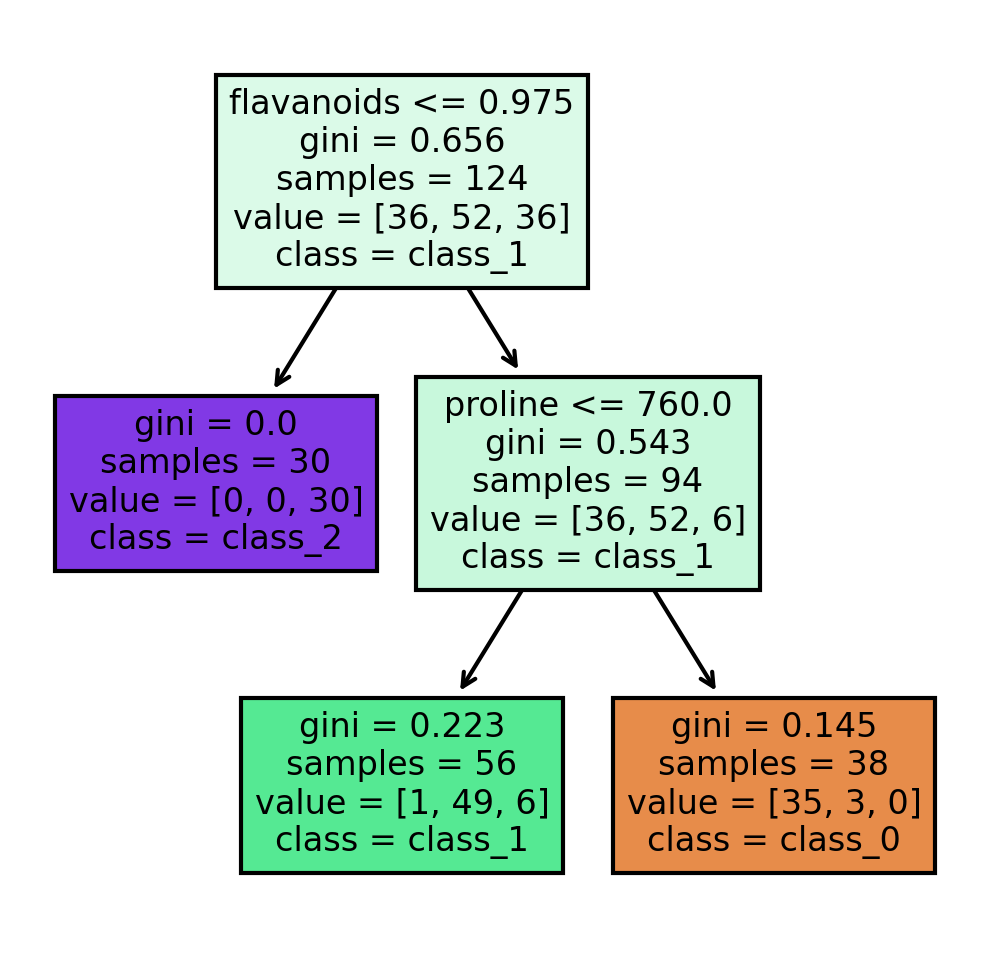
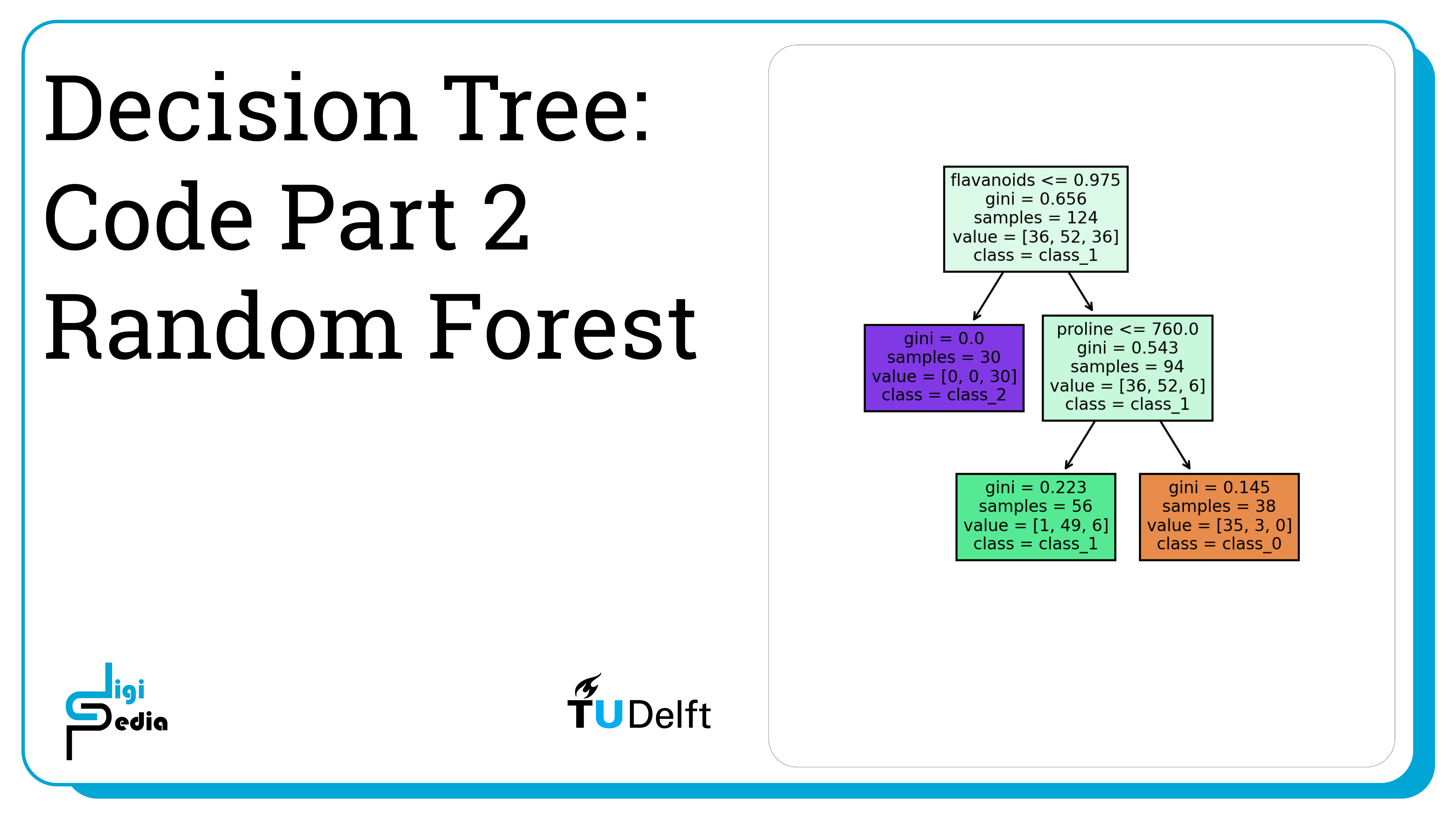
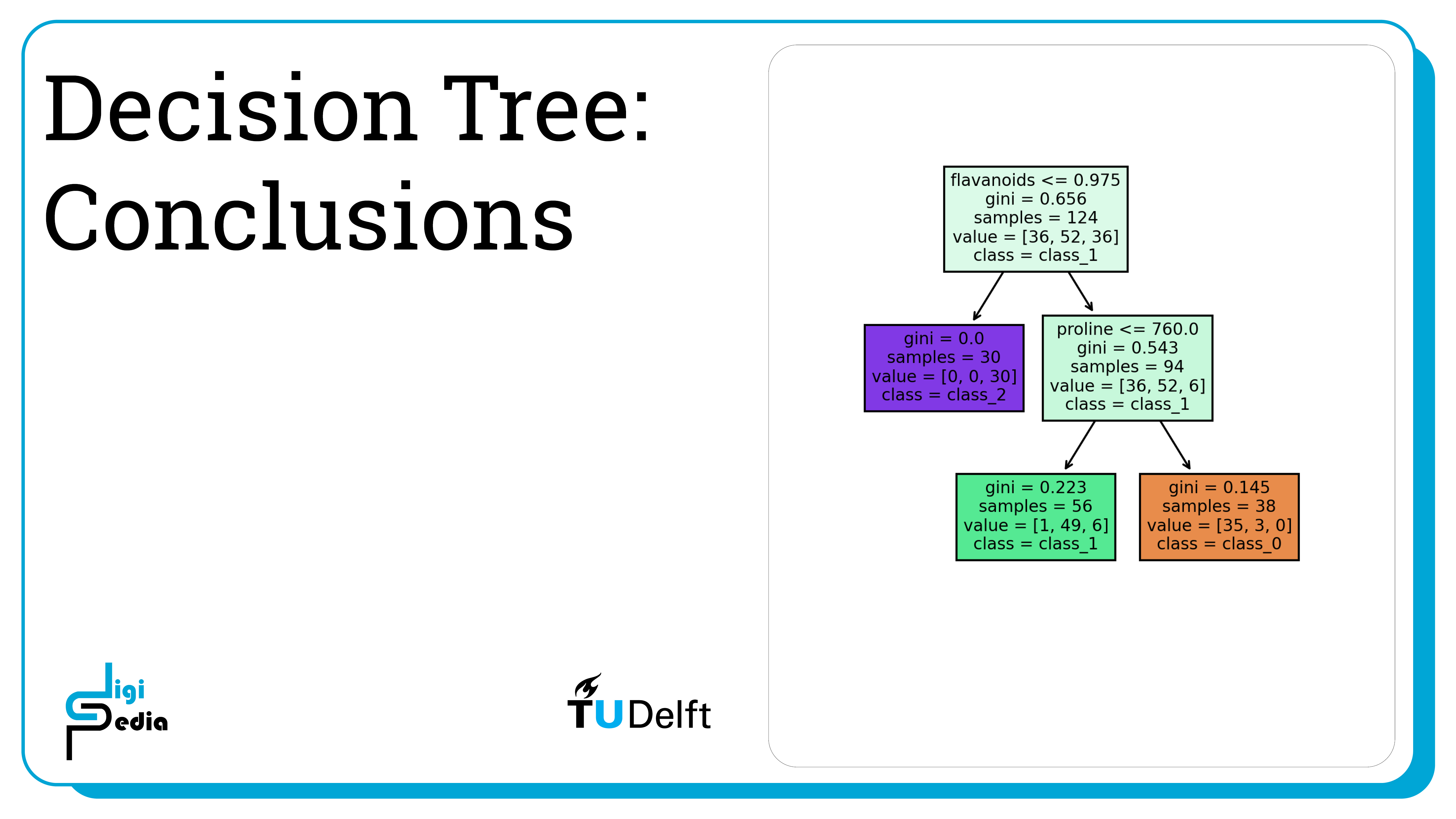
The plot_tree function allows us to plot a visualization of the decision tree generated by the trained classifier. The decision tree stopped splitting after a depth of 2 has been reached. When no maximum depth is set, the tree stops splitting into descendant nodes when the Gini impurity measure is 0. The challenge of not setting a depth is that overfitting can occur.
import matplotlib.pyplot as plt
from sklearn import tree

# Setting dpi = 300 to make image clearer than default
fig, axes = plt.subplots(nrows = 1,ncols = 1,figsize = (4,4), dpi=300)
tree.plot_tree(clf,
          feature_names = wine.feature_names,
      class_names=wine.target_names,
     filled = True);
Random Forest / Decision Trees 3/4
Random Forestlink copied
Creating a Random Forest Classifier
Decision trees have high variance. Even a small change in the training data can result in a drastically different tree. Even the Decision Trees with the highest accuracy, may fail to predict the class of a new datapoint. To address these challenges, Random Forest trains many decision tree classifiers and combines them to predict the class of a new datapoint. Each tree in the Random Forest predicts the class of the new datapoint and the prediction with the most votes becomes the predicted classification. We can see that the accuracy increases when Random Forest is implemented.
The number of trees used in Random Forest Classification with SciKit is defined by the n_estimators hyperparameter. By default, the value is 100, but it can be changed by setting a new value. The example below uses 50 trees.
from sklearn.ensemble import RandomForestClassifier
from sklearn.datasets import make_classification

# Train Random Forest Classifier
clf = RandomForestClassifier(max_depth=2, random_state=0, n_estimators=50)
clf.fit(X_train,y_train)

# Predict the response for test dataset
y_pred = clf.predict(X_test)
print(y_pred)
The output is:
[2 1 0 1 0 2 1 0 2 1 0 0 1 0 1 1 2 0 1 0 0 1 2 0 0 2 0 0 0 2 1 2 2 0 1 1 1 1 1 0 0 1 2 0 0 0 1 0 0 0 1 2 2 0]
# Model Accuracy, how often is the classifier correct?print("Accuracy:",metrics.accuracy_score(y_test, y_pred))

# Which classes are commonly misclassified?
print('Confusion Matrix')
print(metrics.confusion_matrix(y_test, y_pred, labels=None))
The output is:
Accuracy: 0.9814814814814815
Confusion Matrix
[[23 0 0]
[ 1 18 0]
[ 0 0 12]]
Random Forest / Decision Trees 4/4
Conclusionslink copied
- Decision Trees classify data which cannot be linearly separated
- Gini impurity or entropy impurity can be used to measure how homogeneous the data classes in a node are, but Gini impurity is most common because it is less computationally intensive
- A Decision Tree stops splitting when the impurity of a node is 0 or when the samples assigned to a node are small enough or when the maximum tree depth is reached
- Overfitting can often happen when a decision tree is too large
- Plot the misclassification cost against different maximum depth values to understand an acceptable max_depth value
- Random Forest trains many Decision Trees and predicts the classification that receives the most votes to overcome the high variance of individual Decision Trees
Write your feedback.
Write your feedback on "Random Forest / Decision Trees"".
If you're providing a specific feedback to a part of the chapter, mention which part (text, image, or video) that you have specific feedback for."Thank your for your feedback.
Your feedback has been submitted successfully and is now awaiting review. We appreciate your input and will ensure it aligns with our guidelines before it’s published.
