Neural Networks
-
Intro
-
Overview
-
Model and Performance
-
Loss Function
-
Conclusions
Information
| Primary software used | Jupyter Notebook |
| Course | Computational Intelligence for Integrated Design |
| Primary subject | AI & ML |
| Secondary subject | Machine Learning |
| Level | Intermediate |
| Last updated | November 19, 2024 |
| Keywords |
Responsible
| Teachers | |
| Faculty |
Neural Networks 0/4
Neural Networks
A description of neural networks.
Neural networks are computational models inspired by the human brain’s structure and function, designed to recognize patterns and make predictions by learning from data. They consist of interconnected layers of nodes, or “neurons,” that process input data and adjust their connections through training to improve accuracy. Neural networks are the foundation of many advanced machine learning applications, including image recognition, natural language processing, and autonomous systems.
For this tutorial you need to have installed Python, Jupyter notebooks, and some common libraries including Scikit Learn. Please see the following tutorial for more information.
Download the Jupyter notebook here to follow along with the tutorial.
Neural Networks 1/4
Overviewlink copied
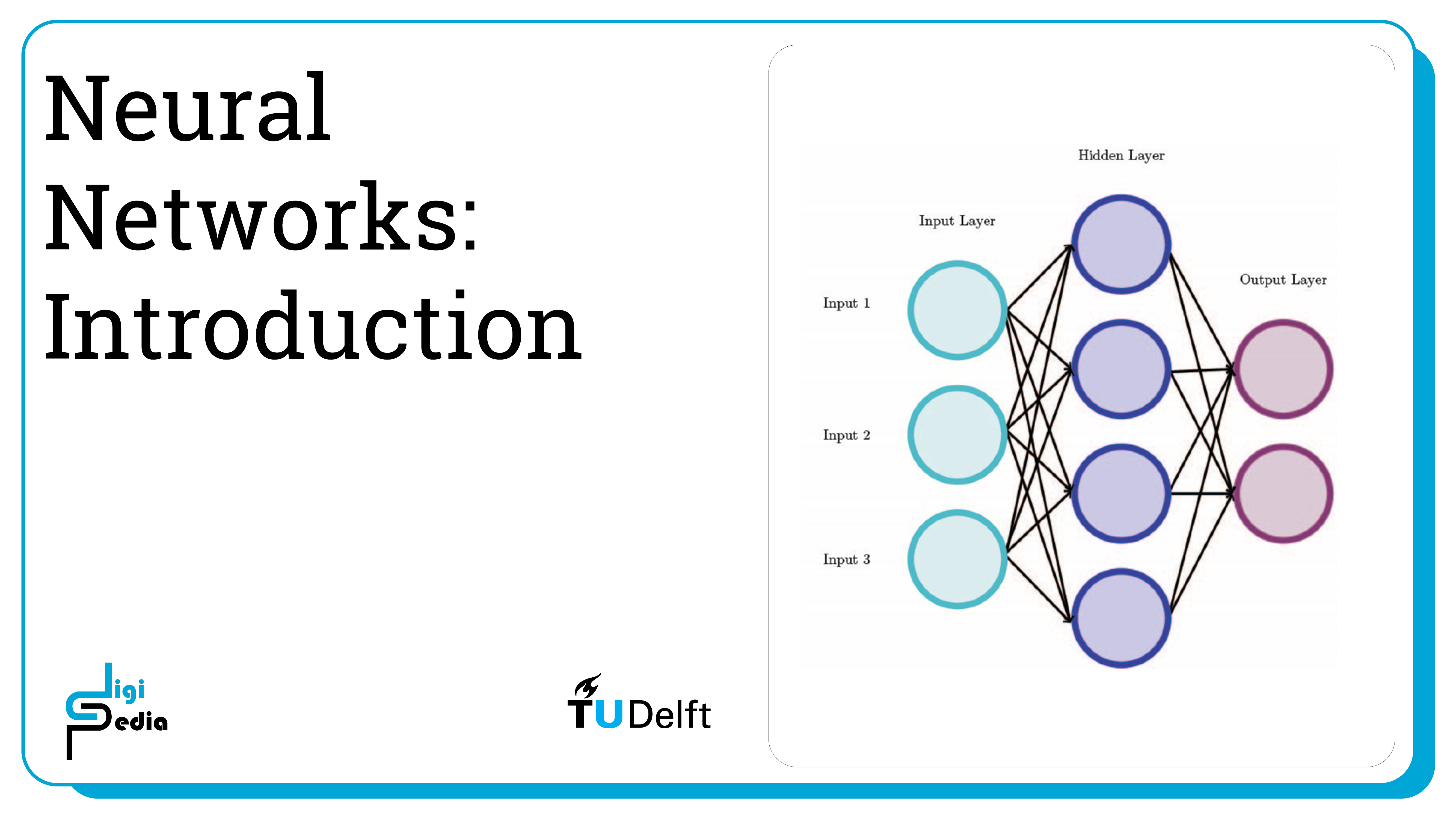
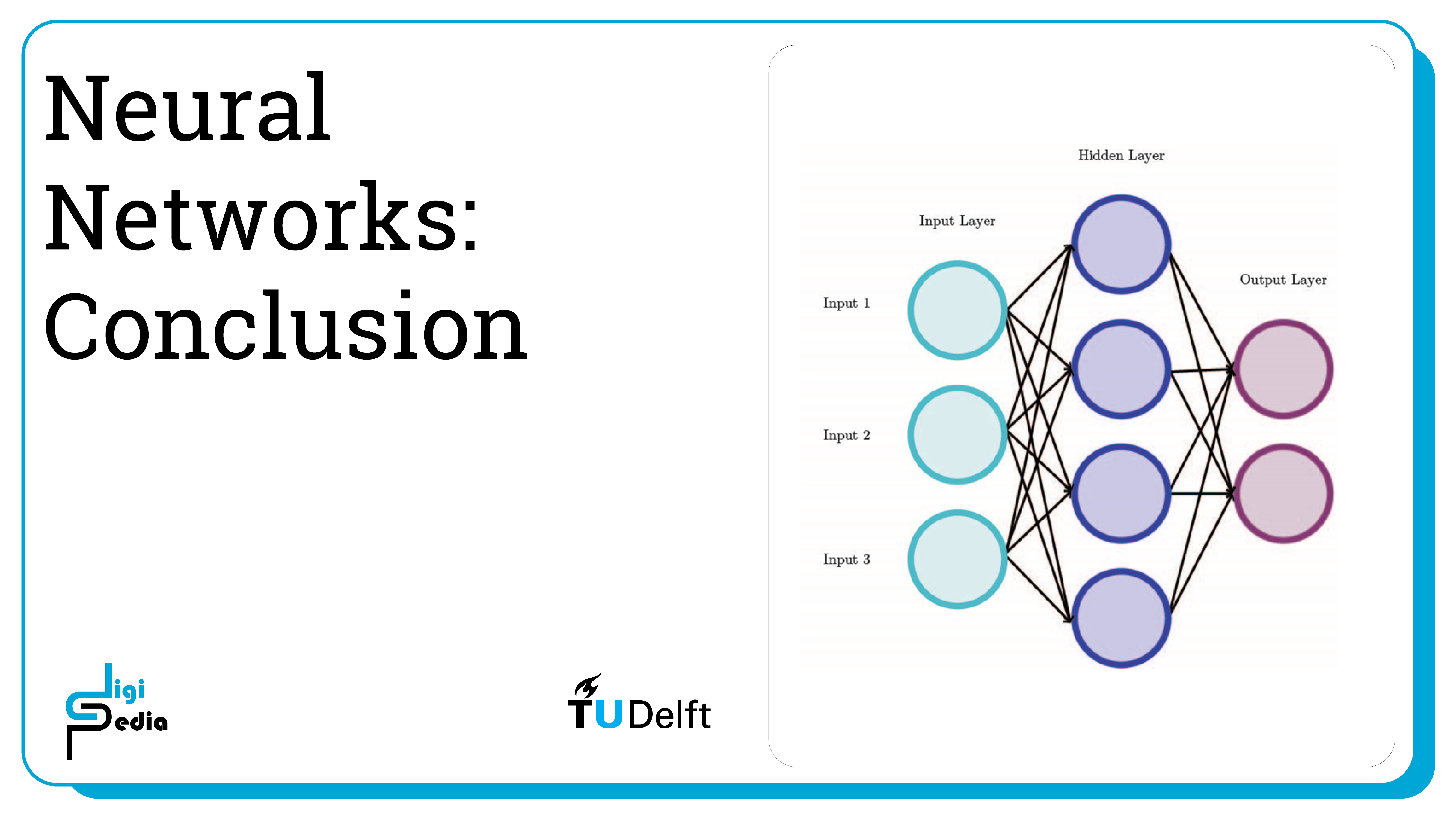
A feedforward neural network also known as a multi-layer perceptron (MLP), is a neural network with at least three layers: an input layer, a hidden layer, and an output layer. A neural network consists of nodes and the connection between the nodes.
Initially, each node was a perceptron with binary output, but contemporarily they consist of activation functions where the output type varies. First, let’s discuss perceptrons.
Perceptrons
A perceptron is the building block of neural networks and is sometimes referred to a single-layer perceptron to distinguish it from an MLP. A perceptron is a threshold function which is a linear classifier. The threshold function maps an input x to an output value f(x). It is the simplest feed-forward neural network. A simplified notation for the threshold function of a perceptron is as follows:
f(x) = 0 if w · x + b ≤ 0, and f(x) = 1 if w · x + b > 0
where w is the weight and b is the bias. The bias value determines how easy it is for a neuron to output a value of 1.
Multi-Layer Perceptron (MLP)
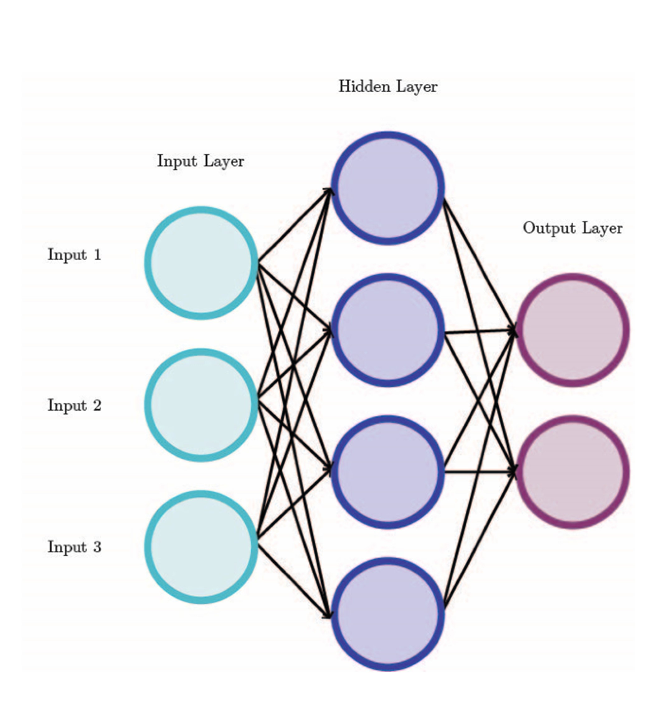
In an MLP, perceptrons are combined in a minimum of three layers. However, when the weight and biases change, the output of a perceptron changes drastically (from 0 to 1 or vice versa). Having a less drastic change in the output and having the output represent a continuous-valued function (for example a value between 0 and 1) provides more accuracy and functionality. Because of this, contemporary neural networks use non-linear activation functions. Each node is not a perceptron anymore but a node with an activation function. Some common activation functions include: sigmoid, TanH, Rectified Linear Unit (ReLU), Leaky ReLU, Exponential Linear Unit (ELU), and SoftPlus. When building a neural network, it is necessary to choose an activation function. In practice the ReLu function is most common.
At the connection between nodes, the output value is multiplied by a weight and a bias is added. The result becomes the input for the next node. MLP learn by changing the weights based on the error in the output when it is compared to the expected result. This is carried out through backpropagation (more about this will be discussed later).
Each of the three types of layers in an MLP use activation functions but the type of layers uses a different function. The input layers uses a linear function. Typically, the nodes in the hidden layer(s) all use the same activation function. Hidden layers also require some design. The number of hidden layers and the number of nodes in each hidden layer need to be determined when building a neural network. There are some rules of thumb to follow for selecting this information, but there is some trial and error involved in seeing how well the neural network performs and adding more layers and nodes as needed.
The nodes in the output layer typically use a different activation function than that used in the hidden layers.
Backpropogation
As mentioned, backpropagation is the algorithm used to train feedforward neural networks. Backpropagation is based on the chain rule, and it only makes sense when nonlinear activation functions are involved. The algorithm starts at the last layer and iterates backwards one layer at a time. Using the chain rule, it calculates the gradient of the loss function with respect to each weight.
Neural Networks 2/4
Model and Performancelink copied
Load Dataset
First we load the data set and visualize some features. See the Jupyter notebook for the output of the print statements.
# Import scikit-learn dataset library
from sklearn import datasets

# Load dataset
wine = datasets.load_wine()

# print the names of the 13 features
print("Features: ", wine.feature_names) # print the label type of wine(class_0, class_1, class_2) print("Labels: ", wine.target_names)

# print the shape of the data set
data(feature)shape wine.data.shape
Train Model
# Import train_test_split function
from sklearn.model_selection import train_test_split

# Split dataset into training set and test set
X_train, X_test, y_train, y_test = train_test_split(wine.data, wine.target, test_size=0.3,random_state=109) # 70% training and 30% test
from sklearn.preprocessing import StandardScaler
scaler = StandardScaler()
# Fit only to the training data
scaler.fit(X_train)
# Now apply the transformations to the data:
X_train = scaler.transform(X_train)
X_test = scaler.transform(X_test)
from sklearn.neural_network import MLPClassifier

mlp = MLPClassifier(hidden_layer_sizes=(50,50,50), activation='relu', solver='adam', max_iter=200)
mlp.fit(X_train,y_train)

predict_train = mlp.predict(X_train)
predict_test = mlp.predict(X_test)

print(predict_test)
The output is:
[0 0 1 2 0 1 0 0 1 0 1 1 2 2 0 1 1 0 0 1 2 1 0 2 0 0 1 2 0 1 2 1 1 0 1 2 0 2 2 0 2 0 0 0 0 2 2 0 1 1 2 1 0 2]
Model Performance
To evaluate the performance of a neural network, it is possible to use similar metrics to those used before like checking the accuracy and printing a confusion matrix. Through SciKit Learn, it is also possible to get the precision, recall, and f1-score of each class.
Precision
- Precision: is the number of true positive results divided by the total predicted positive values
- The total predicted positive values is the sum of the number of true positive results and the false positive results
- For multiple classes, it is the number of correctly classified samples of that class divided by the total number of samples that the classifier assigned to that class
Recall
- Recall: is the number of true positive results divided by the total number of positive results
- The total positive results is the sum of the number of true positive results and the false negative results
- For multiple classes, it is the number of correctly classified samples of that class divided by the total number of samples that actually belong to that class
F-score
- F-score is equal to two times the precision times the recall divided by the precision plus the recall
mlp.score(X_test, y_test)The output is:
0.9629629629629629
# Performance on training dataset
from sklearn.metrics import classification_report,confusion_matrix
# import required modules
import numpy as np
import matplotlib.pyplot as plt
import seaborn as sns
import pandas as pd

class_names=[0,1,2] # name of classes
fig, ax = plt.subplots()
tick_marks = np.arange(len(class_names))
plt.xticks(tick_marks, class_names)
plt.yticks(tick_marks, class_names)

# create heatmap
sns.heatmap(pd.DataFrame(confusion_matrix(y_train,predict_train)), annot=True, cmap="YlGnBu" ,fmt='g')
ax.xaxis.set_label_position("top")
plt.tight_layout()
plt.title('Confusion matrix', y=1.1)
plt.ylabel('Actual label')
plt.xlabel('Predicted label')

print(classification_report(y_train,predict_train))
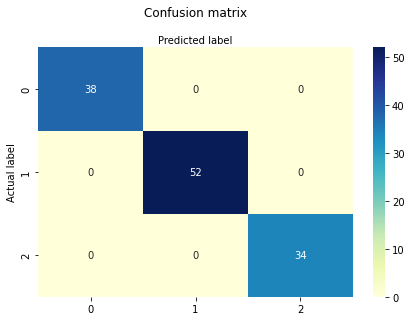
| class | precision | recall | f1-score | support |
| 0 | 1.00 | 1.00 | 1.00 | 38 |
| 1 | 1.00 | 1.00 | 1.00 | 52 |
| 2 | 1.00 | 1.00 | 1.00 | 34 |
| accuracy | 1.00 | 124 | ||
| macro avg | 1.00 | 1.00 | 1.00 | 124 |
| weighted avg | 1.00 | 1.00 | 1.00 | 124 |
Performance on Test Data Set
from sklearn.metrics import classification_report,confusion_matrix

# import required modules
import numpy as np
import matplotlib.pyplot as plt
import seaborn as sns
import pandas as pd

class_names=[0,1,2] # name of classes
fig, ax = plt.subplots()
tick_marks = np.arange(len(class_names))
plt.xticks(tick_marks, class_names)
plt.yticks(tick_marks, class_names)

# create heatmap
sns.heatmap(pd.DataFrame(confusion_matrix(y_test,predict_test)), annot=True, cmap="YlGnBu" ,fmt='g')
ax.xaxis.set_label_position("top")
plt.tight_layout()
plt.title('Confusion matrix', y=1.1)
plt.ylabel('Actual label')
plt.xlabel('Predicted label')

print(classification_report(y_test,predict_test))
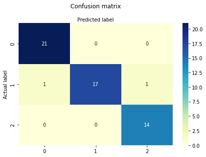
| class | precision | recall | f1-score | support |
| 0 | 0.95 | 1.00 | 0.98 | 21 |
| 1 | 1.00 | 0.89 | 0.94 | 19 |
| 2 | 0.93 | 1.00 | 0.97 | 14 |
| accuracy | 0.96 | 54 | ||
| macro avg | 0.96 | 0.96 | 0.96 | 54 |
| weighted avg | 0.97 | 0.96 | 0.96 | 54 |
Loss Curve
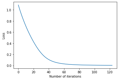
SciKit Learn also tracks the loss curve along the training iterations. By plotting the loss against the iterations, it is possible to visualize if the model is learning. If the loss curve decreases first quickly, and then more slowly like the one below, the neural network is learning. If the loss curve jumps between high and low values or starts by decreasing and then jumps between high and low values, there may be problems with the model (for example, maybe the learning rate is too high) or with the data set (for example, too many outliers or noise in your data set).
import matplotlib.pyplot as plt

fig, ax = plt.subplots(figsize=(6,4))
ax.plot(mlp.loss_curve_)
ax.set_xlabel('Number of iterations')
ax.set_ylabel('Loss')
plt.show()
Neural Networks 3/4
Loss Functionlink copied
Another way to see accuracy of training process
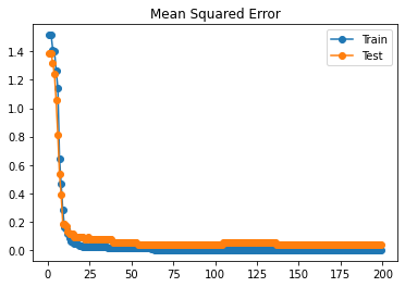
SciKit Learn does not track the accuracy of the training and testing data separately, but when you track these for each iteration and add them to a list it is possible to plot these two metrics at the end. When the curves are similar, it shows that the weights and biases used apply well to the training data and the test data. Additionally, you can track the mean squared error for each iteration and add them to a list to also plot the mean squared error of the train and test data against the training iteration.
from sklearn.metrics import accuracy_score, mean_squared_error

# define lists to collect scores
train_scores, test_scores = list(), list()
mse_train_scores, mse_test_scores = list(), list()

epochs = [i for i in range(1, 200)]
# evaluate for each iteration over 150 iteration

# configure the model
mlp2 = MLPClassifier(hidden_layer_sizes=(50,50,50), activation='relu', solver='adam', max_iter=200, batch_size="auto")
for epoch in epochs:
# fit model on the training dataset
mlp2 = mlp2.partial_fit(X_train, y_train, wine.target)

# evaluate on the train dataset
train_output = mlp2.predict(X_train)
train_acc = accuracy_score(y_train, train_output)
mse_train_acc = mean_squared_error(y_train, train_output)
mse_train_scores.append(mse_train_acc)
train_scores.append(train_acc)

# evaluate on the test dataset
test_output = mlp2.predict(X_test)
test_acc = accuracy_score(y_test, test_output)
mse_test_acc = mean_squared_error(y_test, test_output)
mse_test_scores.append(mse_test_acc)
test_scores.append(test_acc)

# summarize progress
print('>%d, train: %.3f, test: %.3f' % (epoch, train_acc, test_acc))
See the jupyter notebook for the output.
Now that we recorded it, we can plot the data and visualize the precision and mean squared error curves.
Visualize Precision
plt.plot(epochs, train_scores, '-o', label='Train')
plt.plot(epochs, test_scores, '-o', label='Test')
plt.title('Precision') plt.legend() plt.show()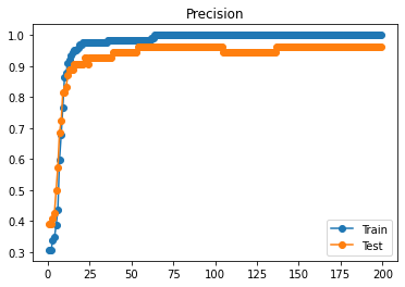
Visualize Mean Squared Error
plt.plot(epochs, mse_train_scores, '-o', label='Train')
plt.plot(epochs, mse_test_scores, '-o', label='Test')
plt.title('Mean Squared Error')
plt.legend()
plt.show()
TASK 1: Find a method or write a method yourself to do 5-fold cross validation with the training data.
TASK 2: Experiment with the neural network architecture. For example, change the depth or the width to improve the accuracy to be above 95%.
Neural Networks 4/4
Conclusionslink copied
- Neural Networks were originally composed of perceptrons which output a binary value
- Contemporary neural networks use nodes with non-linear activation functions instead to output non-binary values
- Common activation functions include: sigmoid, TanH, Rectified Linear Unit (ReLU), Leaky ReLU, Exponential Linear Unit (ELU), and SoftPlus
- Neural networks are trained by adjusting the weights and biases through a process called backpropagation
- Backpropagation starts at the last layer and iterates backwards one layer at a time. Using the chain rule, it calculates the gradient of the loss function with respect to each weight.
Write your feedback.
Write your feedback on "Neural Networks"".
If you're providing a specific feedback to a part of the chapter, mention which part (text, image, or video) that you have specific feedback for."Thank your for your feedback.
Your feedback has been submitted successfully and is now awaiting review. We appreciate your input and will ensure it aligns with our guidelines before it’s published.
