K-Means Clustering
-
Intro
-
Overview
-
Implementing K-Means
-
Conclusions
Information
| Primary software used | Jupyter Notebook |
| Course | K-Means Clustering |
| Primary subject | AI & ML |
| Secondary subject | Machine Learning |
| Level | Intermediate |
| Last updated | November 15, 2024 |
| Keywords |
Responsible
| Teachers | |
| Faculty |
K-Means Clustering 0/3
K-Means Clustering
K-Means clustering is an unsupervised learning algorithm that partitions data into a predefined number of clusters by minimizing the variance within each cluster. It iteratively assigns each data point to the nearest cluster center, recalculates the cluster centers based on the current assignments, and repeats this process until the cluster centers stabilize.
For this tutorial you need to have installed Python, Jupyter notebooks, and some common libraries including Scikit Learn. Please see the following tutorial for more information.
Download the Jupyter notebook here to follow along with the tutorial.
K-Means Clustering 1/3
Overviewlink copied
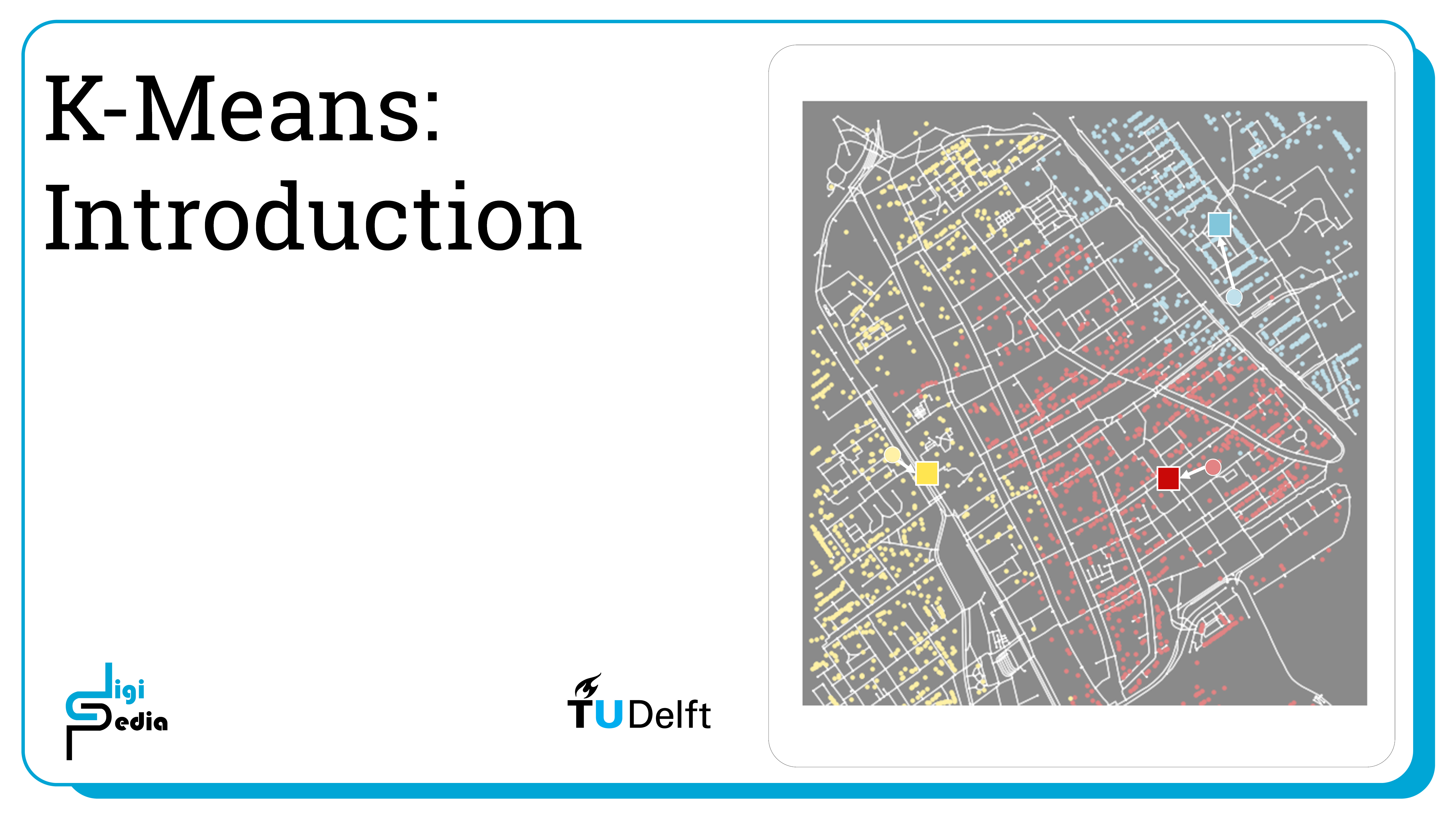
K-Means clustering randomly initializes k cluster centroids in the dataset. Then, the algorithm measures the distance between each cluster centroids and each data point in the data set. The distance metric used can be Euclidean or Manhattan distance. The data points are then assigned to the centroids that is closest to that point.
When all points are assigned, new centroids of the cluster are located by averaging all the datapoints that are assigned to that cluster. The new centroids are then used to repeat the process (measure distance to all points, cluster point to closest centroids, computer new centroids, repeat).
This process continues until a stopping condition is reached. The stopping condition is usually met when a certain number of iterations has been reached, or if the movement of the new centroids point is less than a specific threshold, or if the centroids stop moving. On data that have a structure that allows for clustering, k-means typically converges after a low number of iterations.
K-Means always requires declaring the number of clusters up front. Below, we will discuss methods for determining and optimal k value.
The following image summarizes K-means clustering: 1a. Randomly initialize *k* cluster centroids, 1b. Measure the distance between each point and the cluster 2. Group data points to the nearest cluster 3. Average the points in a cluster to find the new cluster centroid, repeat steps 1b to 3 until a stopping condition is reached.

K-Means Clustering 2/3
Implementing K-Meanslink copied
Dataset
For this example, we will use a randomly generated dataset. Below, we generate this dataset using the SkiKit Learn methods.
import matplotlib.pyplot as plt
from sklearn.datasets import make_blobs

# create dataset
X, y = make_blobs(
   n_samples=150, n_features=2,
   centers=3, cluster_std=0.5,
   shuffle=True, random_state=0
)

# plot
plt.scatter(
   X[:, 0], X[:, 1],
   c='white', marker='o',
   edgecolor='black', s=50
)
plt.show()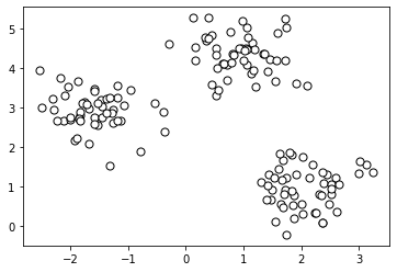
Implement K-Means
from sklearn.cluster import KMeans

clusters = 3

km = KMeans(
    n_clusters=clusters, init='random',
    n_init=10, max_iter=300,
    tol=1e-04, random_state=0
    )
y_km = km.fit_predict(X)
To visualize the result, we can plot the clusters and the centroids using MatPlotLib.To visualize the result, we can plot the clusters and the centroids using MatPlotLib.
# plot the 3 clusters
colors = ['lightgreen', 'orange', 'lightblue', 'lightcoral', 'gold', 'plum', 'midnightblue', ' indigo', 'sandybrown']
markers = ['s', 'H', 'v', 'p', '^', 'o', 'X', 'd', 'P' ]

for i in range(clusters):
    plt.scatter(
        X[y_km == i, 0], X[y_km == i, 1],
        s=50, c=colors[i],
        marker=markers[i], edgecolor='black',
        label='cluster ' + str(i)
    )

# plot the centroids
plt.scatter(
    km.cluster_centers_[:, 0], km.cluster_centers_[:, 1],
    s=250, marker='*',
    c='red', edgecolor='black',
    label='centroids'
)
plt.legend(scatterpoints=1)
plt.grid()
plt.show()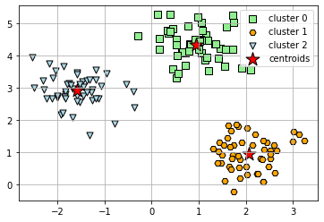
The Elbow Method (to Determine K)
In order to determine the optimal *k* value, it is possible to use an elbow graph. This graph plots the number of clusters against the distortion. The optimal value for *k* is at the ‘elbow’ in the graph. In the graph below, for example we can see that it is 3.
# calculate distortion for a range of number of cluster
distortions = []
for i in range(1, 11):
    km = KMeans(
        n_clusters=i, init='random',
        n_init=10, max_iter=300,
        tol=1e-04, random_state=0
    )
    km.fit(X)
    distortions.append(km.inertia_)

# plot
plt.plot(range(1, 11), distortions, marker='o')
plt.xlabel('Number of clusters')
plt.ylabel('Distortion')
plt.show()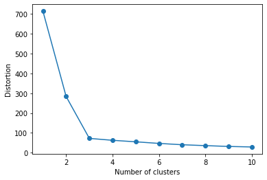
TASK 1: In the classifier below, set n_clusters to 4 by changing the value of the variable “clusters” to 4, and see how the clustering changes.
clusters = 3

km = KMeans(
    n_clusters=clusters, init='random',
    n_init=10, max_iter=300,
    tol=1e-04, random_state=0
)
y_km = km.fit_predict(X)
# plot the 3 clusters
colors = ['lightgreen', 'orange', 'lightblue', 'lightcoral', 'gold', 'plum', 'midnightblue', ' indigo', 'sandybrown']
markers = ['s', 'H', 'v', 'p', '^', 'o', 'X', 'd', 'P' ]
for i in range(clusters):
plt.scatter(
X[y_km == i, 0], X[y_km == i, 1],
s=50, c=colors[i],
marker=markers[i], edgecolor='black',
label='cluster ' + str(i)
)
# plot the centroids
plt.scatter(
km.cluster_centers_[:, 0], km.cluster_centers_[:, 1],
s=250, marker='*',
c='red', edgecolor='black',
label='centroids'
)
plt.legend(scatterpoints=1)
plt.grid()
plt.show()TASK 2: Choose two features from the wine dataset which are appropriate for clustering and apply K-Means clustering on the data based on those two features.
Don’t forget to normalize the input data using a pipeline like we have done in previous notebooks. Check the SVM notebook for an example.
K-Means Clustering 3/3
Conclusionslink copied

- K-means clusters data based on the distance of the data point to a centroid.
- K-means requires knowing how many clusters the result will have.
- The k centroids are randomly initialized, the points are grouped to the nearest centroid, the points are averaged and the centroid is moved to this new location. These steps are repeated until a stopping condition has been reached.
- The features need to be normalized before using them as an input, as it affects the performance of K-Means.
- K-Means does not perform well with non-spherical shapes, unless the data are appropriately transformed beforehand.
Write your feedback.
Write your feedback on "K-Means Clustering"".
If you're providing a specific feedback to a part of the chapter, mention which part (text, image, or video) that you have specific feedback for."Thank your for your feedback.
Your feedback has been submitted successfully and is now awaiting review. We appreciate your input and will ensure it aligns with our guidelines before it’s published.
