Feature Selection
-
Intro
-
Importance of feature selection
-
Preparation
-
Hyperparameters
-
Feature Selection Processes
-
Conclusion
Information
| Primary software used | Python |
| Software version | 1.0 |
| Course | Feature Selection |
| Primary subject | AI & ML |
| Secondary subject | Machine Learning |
| Level | Intermediate |
| Last updated | November 29, 2024 |
| Keywords |
Responsible
| Teachers | |
| Faculty |
Feature Selection 0/5
Feature Selection
xxx
Overview
Machine learning models can be broadly classified as supervised and unsupervised learning. The difference between these two techniques is the structure of the data. Supervised learning requires a labelled data set and unsupervised learning uses unlabelled data.
Regardless of which model is used, the features in your training data are an important consideration to train a reliable model. You want to balance not using too many features, which increases computation time, with having a reliable model, which needs enough meaningful features.
Exercise
During this exercise we are predicting how satisfied people are with their house. To do so we will use random forest classification. To discuss and understand feature selection, we will use a clean version of the following data set:
- The WoOn 2021 survey Citavista – Nieuw (woononderzoek.nl)
Feature Selection 1/5
Importance of feature selectionlink copied
The success of your analysis is depending highly on which variables you select. Variable selection is identifying the impactful features which hold the most information from a dataset. Selecting the right variables leads to better insights of underlying patterns and more accurate predictions.
There are two main takeaways you should keep in mind; the number of features and the feature combination could highly impact the performance.
A higher number of features does not equal a higher performance. Adding features with irrelevant information could cause noise, making it harder to identify truly important information. Additionally, in terms of machine learning, the model could overfit, meaning that the model learns the data too well and being unable to generalise new (unseen) data. This could result in poor predictive performance on new data. In general, it is advisable to select as least features as possible which result in the high performance, as more features require more computational power and therefore more time.
The combination of the selected features matter as the optimal feature combination provides the most relevant information, captures complex relationships and reduces noise and redundancy. Highly correlated features provide similar information and are therefore redundant. It is more effective to select features that are complementary.
Variable selection process
There are several ways to do the process of variable selection:
- exhaustive search
- forward selection
- backward elimination
- information gain
- correlation coefficient
Exhaustive feature search:
Evaluates all possible feature combinations. The exhaustive search strategy is computationally intensive and is time consuming. This is the most optimal search, but also comes with the most downsides. The number of feature combinations that need to be tried is equal to n! (n-factorial), if your data set contains n features. Therefore, more efficient strategies are created.
Forward feature selection:
Based on the relation to target feature the best feature is selected. Then the second best feature in combination with the first feature is added, and so on. This approach gives the best feature combination by adding one feature at a time.
Backward feature elimination:
Based and a target feature the least important feature is eliminated. From the left features the next least important feature is eliminated and so on. The goal is to create a reduced collection of features that are more relevant to the target feature.
Information gain:
Measures how effective a feature is in classifying the target feature. Helps select the features that reduce the uncertainty in the dataset.
Correlation coefficient:
Measures the correlation between each feature and the target feature. The best performing features have minimal correlation with each other and high correlation to the target feature.
Feature Selection 2/5
Preparationlink copied
Loading the dataset
In this case, we will load the clean data set from a CSV file into a Pandas Dataframe. If you need additional information about loading a dataset, review the ‘Cleaning a Data Set’ tutorial which provides more details.
Remember to update the folder location highlighted in blue.

Feature Selection 3/5
Hyperparameterslink copied
We will use a model where the hyperparameters have already been adjusted. If you need additional information about this process, review the “Hyperparameter Turning for Supervised Learning” tutorial which provides more details.
Based on the outcome of this tutorial the tuned hyperparameters for classification are:
- max_depth=6
- max_features=0.45
- n_estimators=200
- random_state=random_int
Feature Selection 4/5
Feature Selection Processeslink copied
Overview
We have already tuned the hyperparameter settings in a separate tutorial. Now, we can test different feature combinations to see how it impacts the success of the model. In this notebook, we will be using a Random Forrest Classifier. The Random Forest algorithm trains a certain number of Decision Trees and uses the most common classification output as the classification for a data point.
Using the models, we can test different feature combinations to see how these impacts the success of the model. The following methods can be used with any machine learning model. Selecting which features should be used to train a model is a long process that is critical to a model’s success. When done successfully, you can use the minimum number of critical features to train an efficient and accurate model. In the following blocks we will see how different combinations of features can impact the model.
For this notebook, we have selected a few different feature selection methods to compare. This is not an exhaustive list, but it provides some examples.
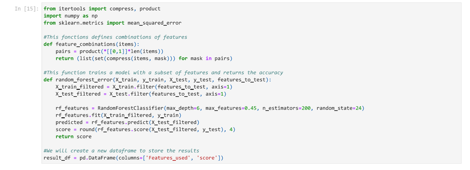
The first cell defines some functions that will be used later in the notebook.
Importance of Feature Selection
As we discussed, you want to use the minimum number of features that provides the best training to balance computational power and model accuracy. This is possible because not all features are created equal. To demonstrate this, we have provided an example.
- First, different combination of the same number features can result in different accuracies.
- Second, it is important to keep in mind that more features aren’t necessarily better.
To demonstrate these concepts, we will train two different models each using four features of our training data set.

We see from these two models, which both use 4 features, that models using the same number of features, but different specific features can have different accuracy. This is because the model is finding corelations in the data between the features and the predicted outcome. If the features do not help to inform the predicted outcome, the model will perform poorly. Additionally, correlations can be found in different combinations of features.
Now we will see if we can improve the accuracy by adding a few more features. We will try 2 different sets of 2 features.

Here we can see that adding features did improve the training when the right combination of features is selected. Not all features are useful. Therefore, testing different combinations can help determine which features are most important for the training.
The combinations of features we used in the above cells were specifically selected for this example. The only way to know which features will impact the accuracy is to test the different combinations. Methods for determining this are discussed in the following sections.
Exhaustive Feature Search
This method trains a model with all possible combinations of features. This is the longest and most computationally intense feature search option. For our data set, where we have so many different features to compare the runtime of this method can be hours or even days. If your data set contains n features, then the number of feature combinations that need to be tried is equal to n! (n-factorial).
To demonstrate how an exhaustive features search would work, we are going to do an exhaustive search of a set of only five features. We will first run the code for the first five features and then for the next five features so we can review the results.
First, see how the code works by running the next block. In the second line, we take only the first 5 features to compare every combination for. This is so the code runs faster but you can still see the results.

Then we can check the next 5 features by running the following cell.
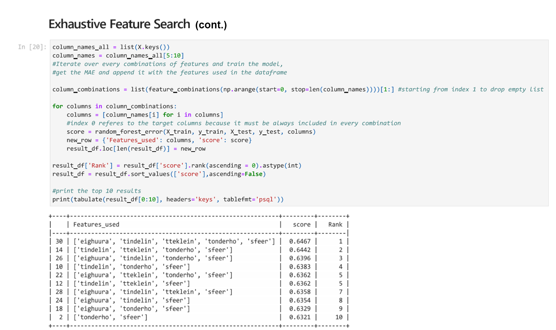
When looking at the results of these two comparisons, we see that of the different combinations tested, using ‘eighuura’, ‘tindelin’, ‘tteklein’, ‘tonderho’, and ‘sfeer’ as the features trains a model with an accuracy of 0.6467. This is the highest of the features that were tested in this small-scale test. We can see that when testing combinations of the first 5 features, that not all features have the same impact.
This shows several things:
First, more features aren’t necessarily better. Some models that used five features had a lower accuracy. It is better to use fewer features when possible because the number of features used impacts the computational power necessary to train the model and therefore the training time.
Second, different combination of features can be equally valuable to predict an outcome. We can see that there are several models that use the same number of features that perform similarly well but use different combinations of features. This is why it is important to review features and test different combinations.
You may have noticed that before we selected a subset of features, our model’s accuracy was higher. This is because we only tested combinations of the first five and second five features. We are looking at the features in small batches so you can run the cells on your computer.
Forward Feature Selection / Backward Feature Elimination
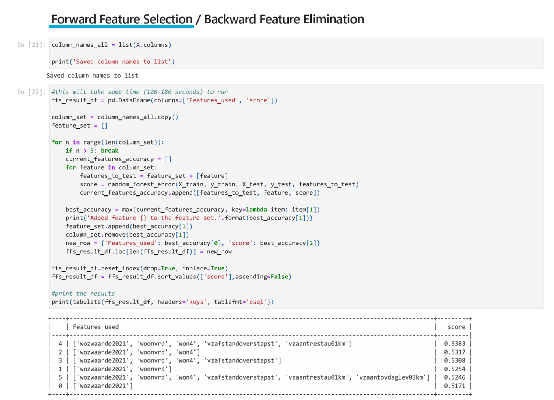
Forward feature selection starts by testing 1 feature. It tests all the features individually and saves the feature that leads to the most accurate model. Then it tests this feature with a second feature. It tests all options for the second feature and again saves the best performing feature to take as the second feature. This continue until the loop stops which is usually until all features have been added so then the best performing set of features can be selected from this longer list.
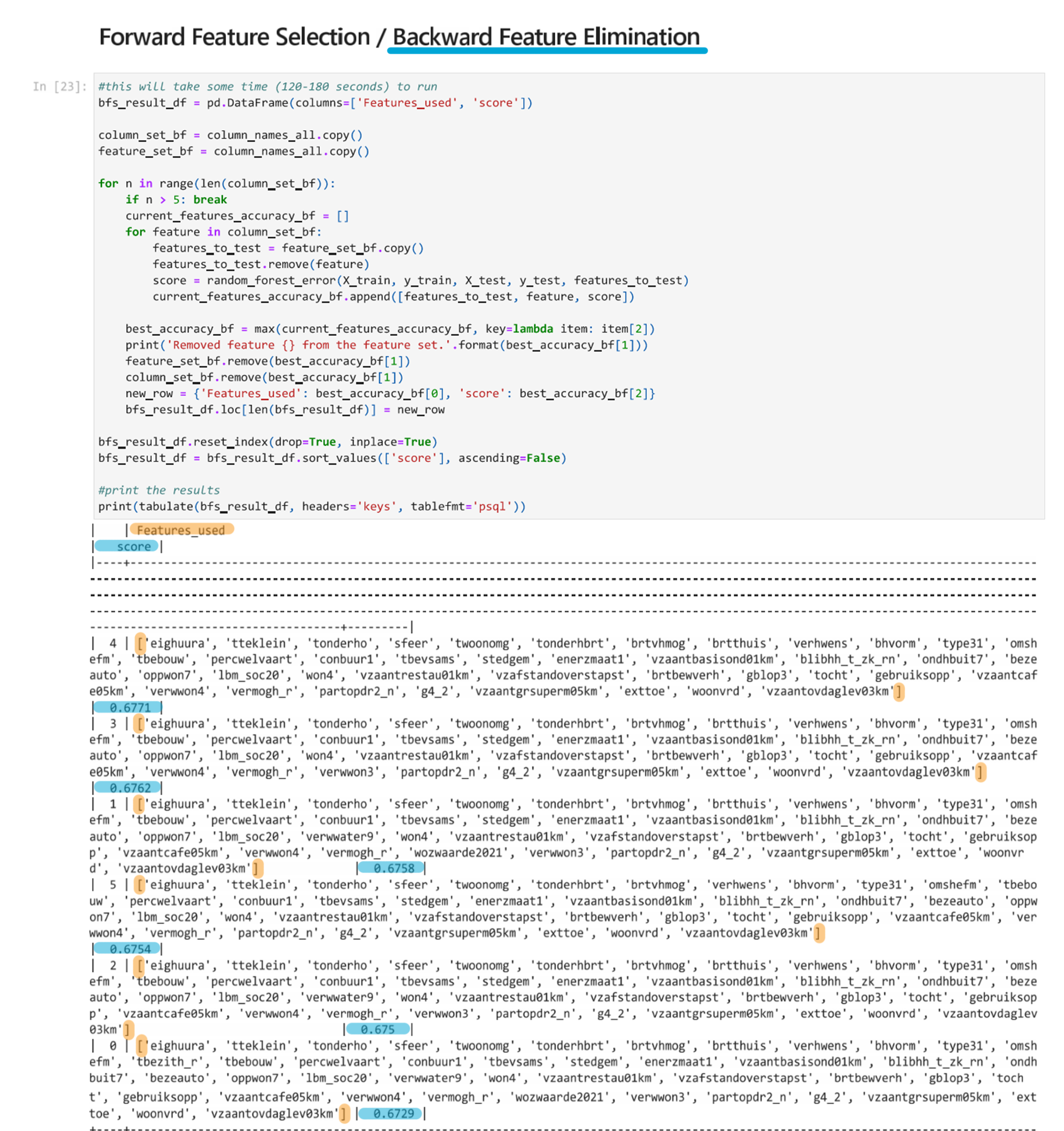
Backward feature elimination does the inverse. It starts will all features and removes one, then another, and another. Each time it tests which feature should be removed to keep the highest accuracy.
Below are the examples of both using only 5 iterations to reduce run time.
Similarly for the first 5 iterations of the backward feature elimination, we can run it and see the results. In the image, the score is highlighted in blue and the parentheses of the list are highlighted in orange to make it easier to read. Please note the highlights are post-processed and will not appear in the Jupyter notebook.
Information Gain
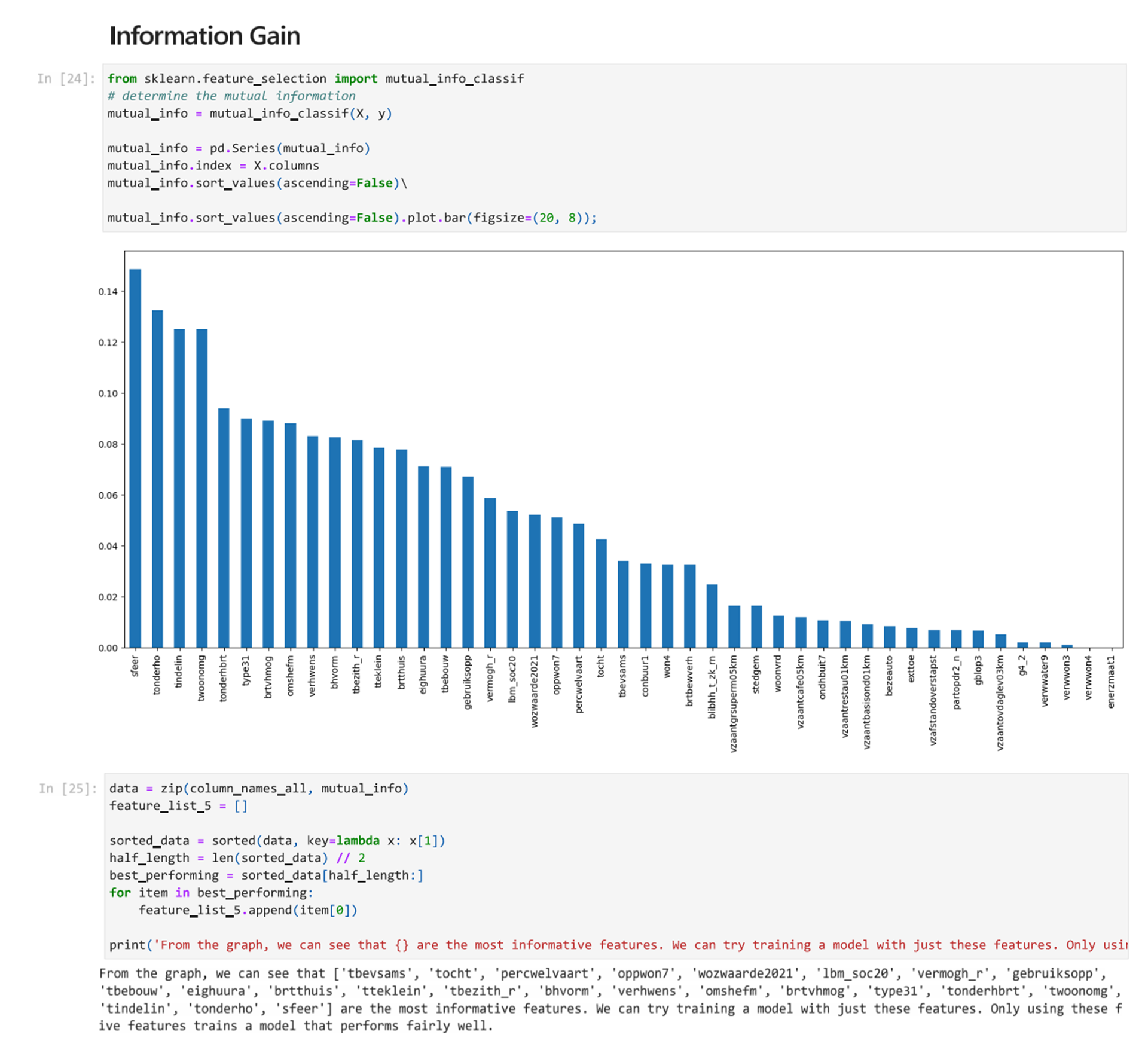
In feature selection, Information Gain (IG) is a measure of how much information a feature provides about a class. It measures the reduction in entropy that is achieved when a data set is split based on a feature. It is then possible to use the information gain measure to select the most informative features for building a model.
Scikit has a function that can measure mutual information, which is the MI Estimate. It measures the dependency between the features. If two random features are independent, it is equal to zero. A higher MI estimate means higher dependency.
By running the cell and plotting the results, we can see an organized list of features that have a large impact on the accuracy.
Correlation Coefficient
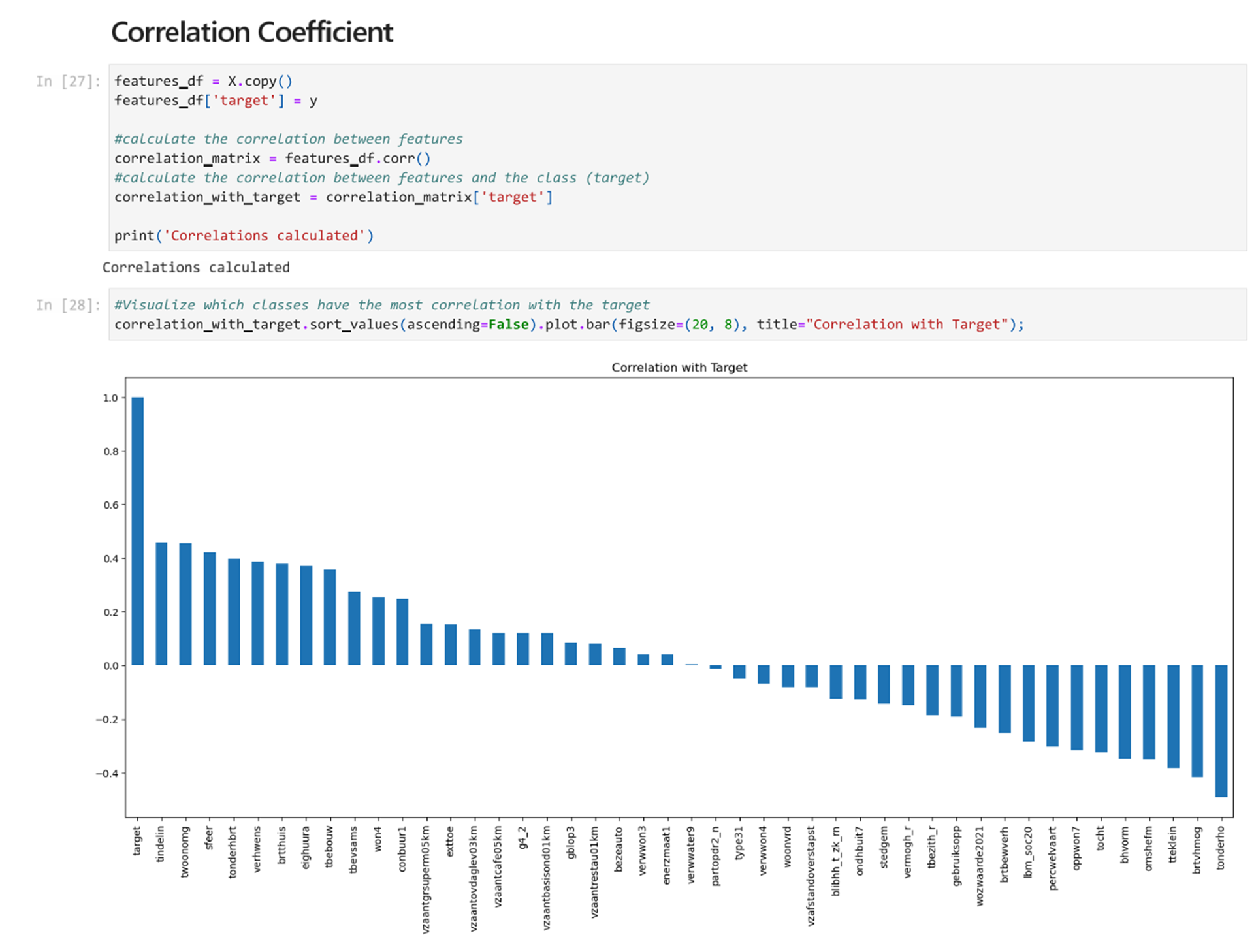
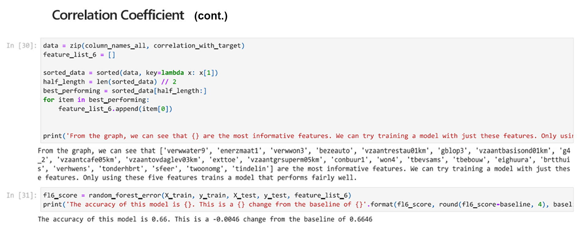
Correlation describes how statistically connected features are to each other and to the class (target). The algorithm used to determine this for features selection is called the Correlation Feature Selection algorithm and it first calculates the correlation between each feature and the class. After this, it calculates the correlation between pairs of features in the features set. The best performing features will have minimal correlation with each other and high correlation to the class that the algorithm will predict. We can plot the correlation coefficient to compare.
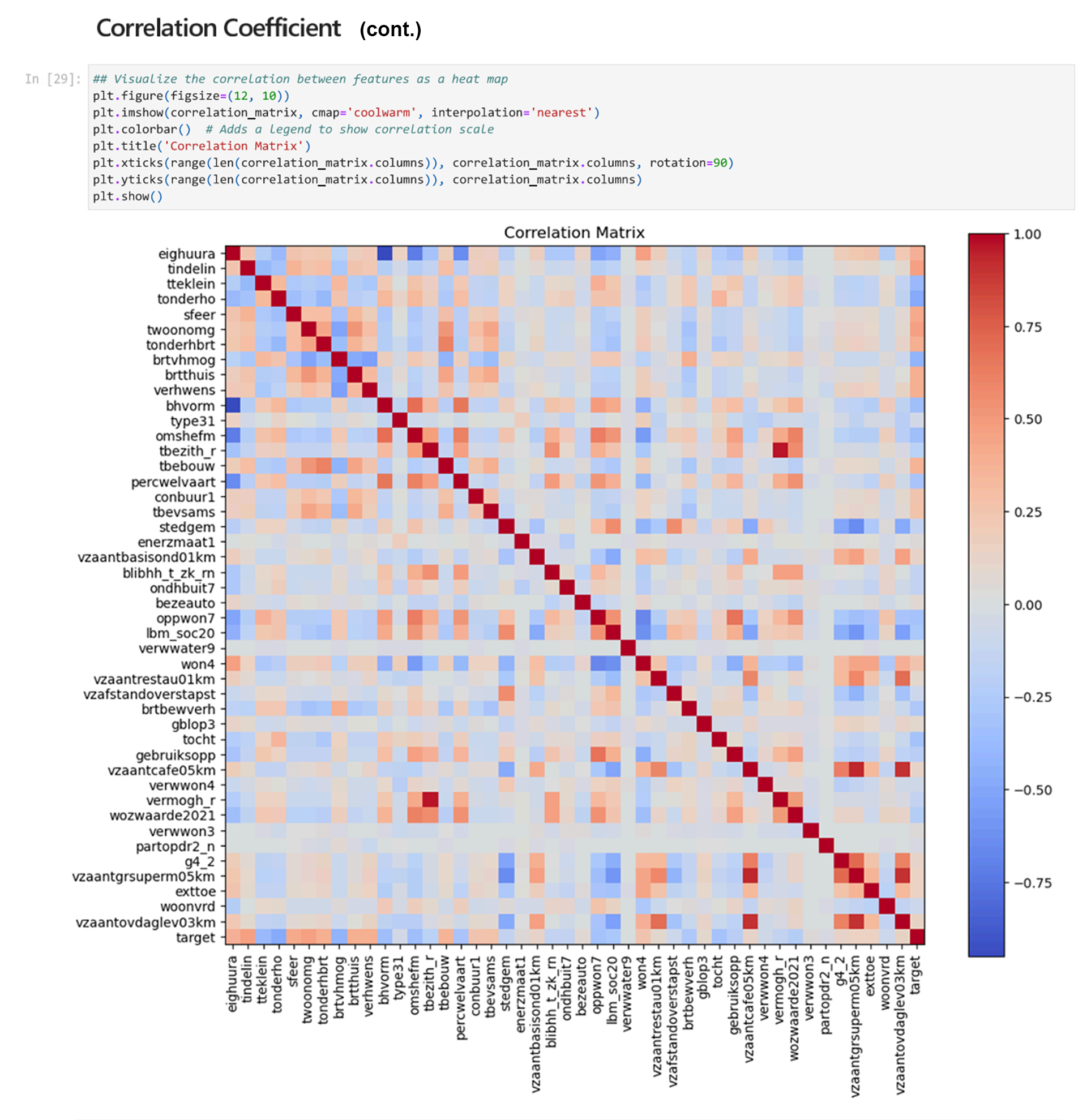
We can also use a heatmap to visualize the corelation between features and the target and features against each other. A red square with a value of 1.0 shows the highest correlation.
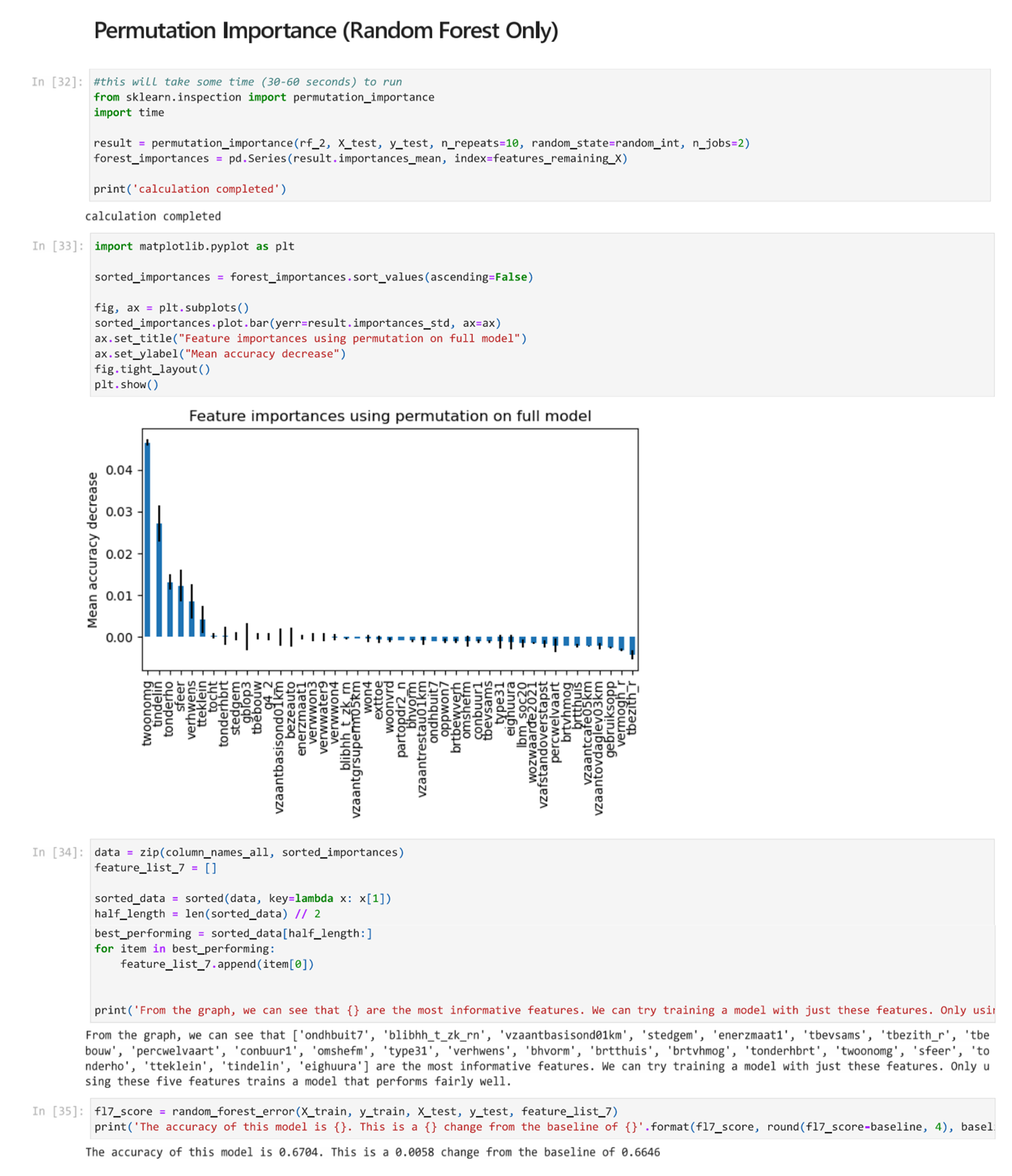
Permutation Importance (Random Forest Only)
Permutation importance measures the importance of different features for a specific trained model. Importantly, it does not reflect to the intrinsic predictive value of a feature by itself but how important this feature is for a particular model. Permutation importance is only relevant for Random Forest models, and it can be a way to check if the features selected had the expected impact.
You can see Permutation Feature Importance Scikit Learn for more information.
Feature Selection 5/5
Conclusionlink copied
Before starting with the feature selection process, it is important to clean your data set and already have a tuned model. Then once features are selected, it is possible to go back and tune the model once more.
We can see through this notebook that there are different methods that can be used to select features for training machine learning models. There are also some methods that have not been described here. From the options shown, many of them require checking combinations of features and this can be time consuming and computationally intensive. However, it is a valuable step as it can reduce training time and improve the accuracy of your model. Achieving the same or slightly better accuracy with significantly fewer features benefits the model.
When selecting features, the notebook has shown that more features aren’t necessarily better and sometimes there may be no or little correlation between features and the prediction you are attempting to make. This means that you cannot predict the outcome you wish with the data you have. It will require the collection of different data to train an accurate model.
Write your feedback.
Write your feedback on "Feature Selection"".
If you're providing a specific feedback to a part of the chapter, mention which part (text, image, or video) that you have specific feedback for."Thank your for your feedback.
Your feedback has been submitted successfully and is now awaiting review. We appreciate your input and will ensure it aligns with our guidelines before it’s published.
