Binary Classification Of 2D Data
-
Intro
-
Generate Dataset
-
Training a Decision Tree
-
Make Predictions
-
Hyperparameters Tuning
-
Visualising the Decision Tree
-
Validating the model
-
Conclusion
Information
| Primary software used | Python |
| Software version | 1.0 |
| Course | Binary Classification Of 2D Data |
| Primary subject | AI & ML |
| Secondary subject | Machine Learning |
| Level | Intermediate |
| Last updated | November 12, 2025 |
| Keywords |
Responsible
| Teachers | |
| Faculty |
Binary Classification Of 2D Data 0/7
Binary Classification Of 2D Data
Example of a double moon shaped point dataset for binary classification.
This tutorial will guide you through the application of a Machine Learning technique called Decision Tree to classify data points based on a predefined set of features. You will use binary classification for data represented by two features only. This will allow us to plot the decision boundary in 2D and visually inspect the model performance. For this exercise, we will use an artificial dataset, i.e. a dataset containing artificially created data points.
After this tutorial you will have a broad understanding of classification in the context of machine learning. You will be able to setup a simple classification problem using Decision Trees, inspect the model performance, plot and interpret the results.
Binary Classification Of 2D Data 1/7
Generate Datasetlink copied
Import Libraries
We will use the sklearn library to artificially generate a 2D binary classification dataset. We start by importing the required libraries for data analysis, machine learning and data visualisation, and generating the dataset.
# import libraries
from google.colab import files
import pandas as pd
import numpy as np
import matplotlib.pyplot as plt
from sklearn.tree import DecisionTreeClassifier
from sklearn.model_selection import train_test_split
from sklearn.datasets import make_moons
from sklearn.metrics import accuracy_score, confusion_matrix, ConfusionMatrixDisplay
The function make_moons produces a data point distribution approximating the shape of two interleaving half circles. Each point is assigned with class 1 or 0.
We pass three arguments to the function:
- n_samples is the number of data points to generate
- noise controls how much the points deviate from the distribution shape
- random_state is a random seed generator. Assigning an integer to this argument will ensure that the dataset will always be the same each time you run this code snippet.
# generate an artificial dataset
featureVector, classVector = make_moons(n_samples=300, noise=0.15, random_state=42)
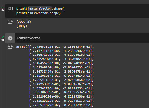
To inspect the data structure of featureVector and classVector, use the method shape and print the result. The result shows that featureVector consists of 300 samples, each one represented by 2 numbers. classVector is instead a 1D vector of 300 samples.
print(featureVector.shape)
print(classVector.shape)
Output:
(300, 2)
(300,)
Visualise the Dataset
We can use the matplotlib library to visualise the data point distribution in 2D. The function scatter allows coloured points on a 2D graph. We assign the values of features 1 and 2 as coordinates x and y, respectively. Then, we assign the values in classVector as colour ‘c’.
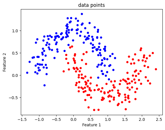
The graph represents how the classes are distributed and demonstrates that the decision boundary we are looking for is non-linear. These two groups of points cannot be separated in the graph by a single straight line.
# plot the dataset
plt.scatter(x = featureVector[:, 0], y = featureVector[:, 1], c=classVector, cmap='bwr', s=20)
plt.title("data points")
plt.xlabel("Feature 1")
plt.ylabel("Feature 2")Binary Classification Of 2D Data 2/7
Training a Decision Treelink copied
In this section we will use the sklearn library to train a Decision Tree Classifier on our dataset. To review what are Decision Trees and how a Decision Tree Classifier works, please refer to the learning material.The DecisionTreeClassifier method takes two arguments:
- max_depth: an integer indicating the depth of the Decision Tree. This corresponds to how many times the tree splits the feature space searching for regions only containing same class data points. (see also ‘Hyperparameters Tuning’)
- random_state: an integer value ensuring that the training process will always start from the same initial random state, allowing to reproduce the results each time the code is ran (see also the ‘Generate Datset’ section)
Note: max_depth is also called an hyperparameter of the Decision Tree.
# Train a decision tree classifier on the geometric dataset
clf_spiral = DecisionTreeClassifier(max_depth=4, random_state=42)
clf_spiral.fit(featureVector, classVector)
Binary Classification Of 2D Data 3/7
Make Predictionslink copied
We can now use the model to make new predictions. For instance, we can a random point in the feature space and ask the model whether it belongs to class 0 or 1. To do so we use the predict method.
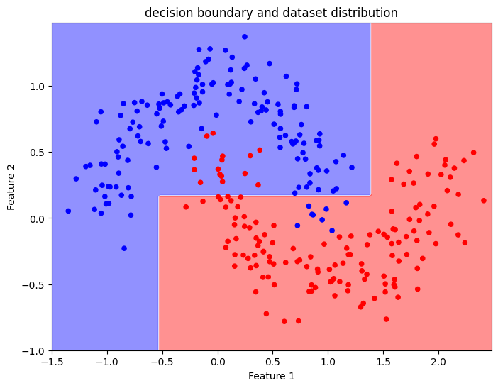
In this example, the model predicts the class 0 for point (0.3,2). If you look back at the dataset distribution graph, you can check whether the model made a good guess.
# single point prediction
new_point = np.array([[0.3,2]])
new_point_class = clf_spiral.predict(new_point)
print(new_point_class)
Output = [0]
Visualise the Decision Boundary
Since our feature space is 2D, we can plot any prediction the model makes on a 2D graph. As with the graphs shown before, every point on this graph has x, and y coordinates corresponding to the input features, whereas colour corresponds to the predicted class. The graph represents the decision boundary, which is the function mapping each data point to one class (refer to the learning material with definitions).
To construct a visualisation of the decision boundary we must first construct a grid of x and y values, to be used as features describing input data points. Then we will use the trained Decision Tree Classifier to predict the class of these points.
# Create a mesh to plot decision boundary for the geometric dataset
xx_range = np.arange(-1.5, 2.5, 0.02)
yy_range = np.arange(-1, 1.5, 0.02)
xx_spiral, yy_spiral = np.meshgrid(xx_range,yy_range)

Z_spiral = clf_spiral.predict(np.c_[xx_spiral.ravel(), yy_spiral.ravel()])
Z_spiral = Z_spiral.reshape(xx_spiral.shape)
We will use the matplotlib contour plot to overlay on our point distribution graph the two regions in the feature space corresponding to the two classes. The polyline separating the two regions is the decision boundary learned by the Decision Tree Classifier.
# plot the decision boundary learned by the Decision Tree
plt.figure(figsize=(8, 6))
plt.contourf(xx_spiral, yy_spiral, Z_spiral, cmap='bwr', alpha=0.5)

# overlay the original data distribution
plt.scatter(x = featureVector[:, 0], y = featureVector[:, 1], c=classVector, cmap='bwr', s=20)
plt.title("decision boundary and dataset distribution")
plt.xlabel("Feature 1")
plt.ylabel("Feature 2")
plt.show()
Binary Classification Of 2D Data 4/7
Hyperparameters Tuninglink copied
The Decision Tree could correctly capture the distribution of the two classes, but the decision boundary is quite coarse.
To improve the Decision Tree performances, we may increase the max_depth parameter to 10 and retrain the model. With a higher number of nodes, we see a more refined decision boundary.
While the boundary is more refined, there is a potential risk of overfitting. This shows how a deeper tree can better approximate the data structure but might lose some generalisation ability.
# Train a decision tree classifier on the geometric dataset
clf_spiral = DecisionTreeClassifier(max_depth=10, random_state=42)
clf_spiral.fit(featureVector, classVector)

# Create a mesh to plot decision boundary for the geometric dataset
xx_range = np.arange(-1.5, 2.5, 0.02)
yy_range = np.arange(-1, 1.5, 0.02)
xx_spiral, yy_spiral = np.meshgrid(xx_range,yy_range)

Z_spiral = clf_spiral.predict(np.c_[xx_spiral.ravel(), yy_spiral.ravel()])
Z_spiral = Z_spiral.reshape(xx_spiral.shape)

# plot the decision boundary learned by the Decision Tree
plt.figure(figsize=(8, 6))
plt.contourf(xx_spiral, yy_spiral, Z_spiral, cmap='bwr', alpha=0.5)

# overlay the original data distribution
plt.scatter(x = featureVector[:, 0], y = featureVector[:, 1], c=classVector, cmap='bwr', s=20)
plt.title("decision boundary and dataset distribution")
plt.xlabel("Feature 1")
plt.ylabel("Feature 2")
plt.show()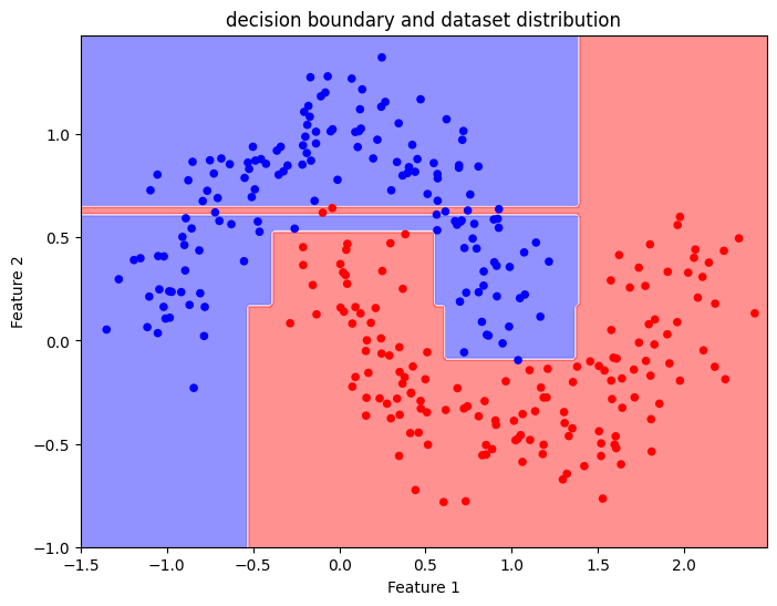
Binary Classification Of 2D Data 5/7
Visualising the Decision Treelink copied
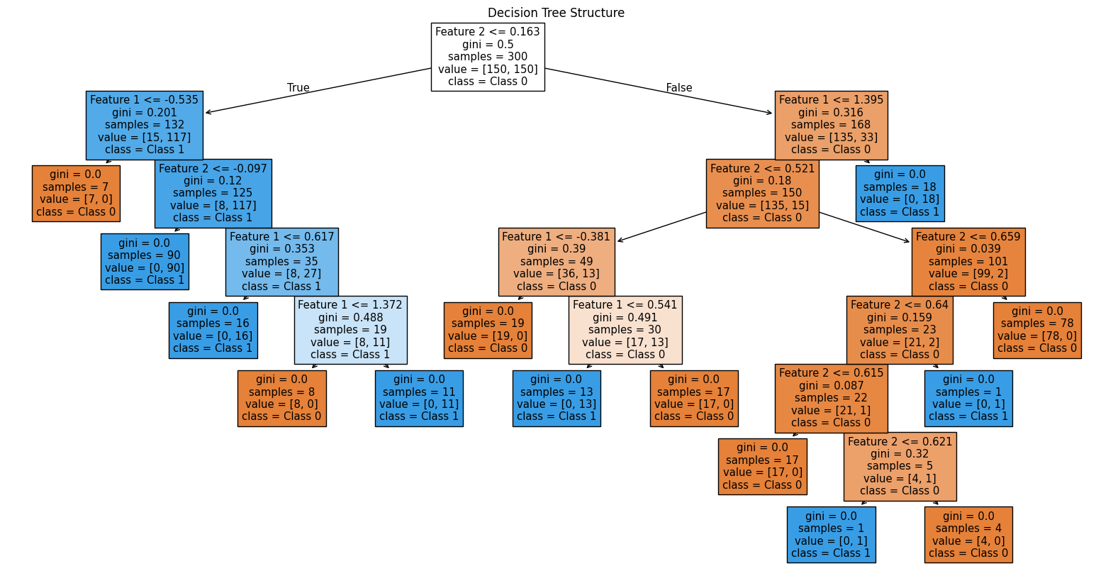
To visualise the structure of the Decision Tree, you can use plot_tree from sklearn.tree. This shows the tree’s splits, decision rules, and leaf nodes, unveiling how the classifier is making decisions.
For our Decision Tree, we note that the outmost nodes, called leaves, are responsible for overfitting. This indicates that a shallower tree could do a better job at generalising.
Binary Classification Of 2D Data 6/7
Validating the modellink copied
Generally, real-world data are high dimensional which makes it impossible to visualise the decision boundary and inspect the model’s performances. Furthermore, we haven’t constructed a performance index yet. This index in classification represents the accuracy of the model.
To validate the model, we will use part of the dataset for training and another for testing. We use the train_test_split module to create the train and test datasets.
Each dataset will contain input vector X and corresponding label y. The parameter test_size controls the % of samples removed from the training dataset for testing.
# Step 1: Split data into train and test sets
X_train, X_test, y_train, y_test = train_test_split(featureVector, classVector, test_size=0.3, random_state=42)

# Step 2: Initialize and train the Decision Tree model
clf_spiral = DecisionTreeClassifier(max_depth=4, random_state=42)
clf_spiral.fit(X_train, y_train)
Compute Accuracy Score
To compute the model’s accuracy, we use the test dataset as input for the trained Decision Tree and obtain the model’s predictions. We then compare the model’s predictions with the correct labels using the method accuracy_score.
In this case the accuracy is 0.9, meaning that the model predicts the correct class of the test dataset 9 out of 10 times.
Try increasing max_depth and observe how accuracy changes.
# Step 3: Predict on test set and measure accuracy
y_pred = clf_spiral.predict(X_test)
accuracy = accuracy_score(y_test, y_pred)
print(f"Test Set Accuracy: {accuracy:.2f}")
>> Test Set Accuracy: 0.90
Plot Confusion Matrix
As a final step we can create a graph to display the confusion matrix. This graph displays how many times the test dataset samples were classified correctly. For instance, the graph shows that 38 samples with class 0 and 43 samples with class 1 were predicted correctly. The model misclassified just 9 samples with class 1 as class 0 (for more details about confusion matrices refer to learning material).
# Step 4: Construct Confusion Matrix
conf_matrix = confusion_matrix(y_test, y_pred)
disp = ConfusionMatrixDisplay(confusion_matrix=conf_matrix, display_labels=clf_spiral.classes_)
disp.plot(cmap="Blues")
plt.title("Confusion Matrix")
plt.show()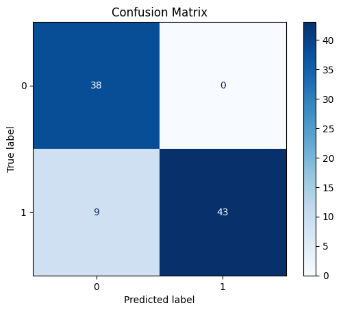
Binary Classification Of 2D Data 7/7
Conclusionlink copied
This tutorial provided you with an overview of classification using Decision Trees, a supervised learning technique for distinguishing between classes based on data features. You learned to set up a classification model, adjust its parameters, and evaluate its accuracy using a test dataset. You also learned about how to visualise the decision boundary in 2D classification problems, refine the model using hyperparameter tuning, and assessing model performance through a confusion matrix.
Exercise File
Here you can find the full Python code which you can open in Google Colab or respective program.
Write your feedback.
Write your feedback on "Binary Classification Of 2D Data"".
If you're providing a specific feedback to a part of the chapter, mention which part (text, image, or video) that you have specific feedback for."Thank your for your feedback.
Your feedback has been submitted successfully and is now awaiting review. We appreciate your input and will ensure it aligns with our guidelines before it’s published.
