3D Grid From Surface
-
Intro
-
3D Grid from Surface
-
BoxMorph
-
Surface Analysis
-
Color by Slope
-
Conclusion
Information
| Primary software used | Grasshopper |
| Course | 3D Grid From Surface |
| Primary subject | Parametric Modeling |
| Secondary subject | General |
| Level | Beginner |
| Last updated | November 11, 2024 |
| Keywords |
Responsible
| Teacher | |
| Faculty |
3D Grid From Surface 0/5
3D Grid From Surface
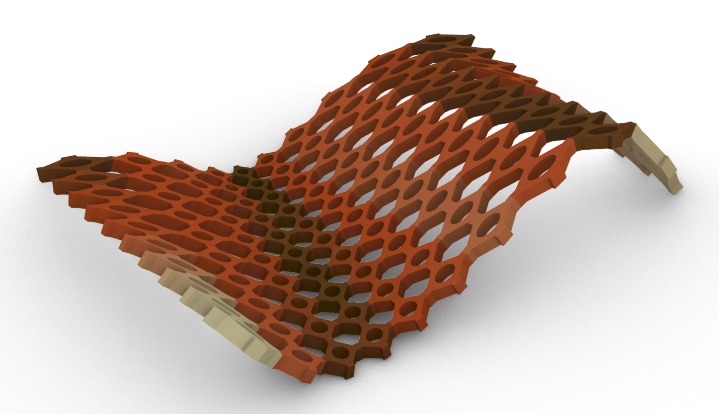
This tutorial is focused on three useful tools in Grasshopper: UV subdivision of surfaces, box morphing and finally coloring based on surface properties
This tutorial is focused on three useful tools in Grasshopper: UV subdivision of surfaces, box morphing and finally coloring based on surface properties. First, we create a lofted surface in Rhino. The surface can be changed by control points along the curves of the loft.
3D Grid From Surface 1/5
3D Grid from Surfacelink copied
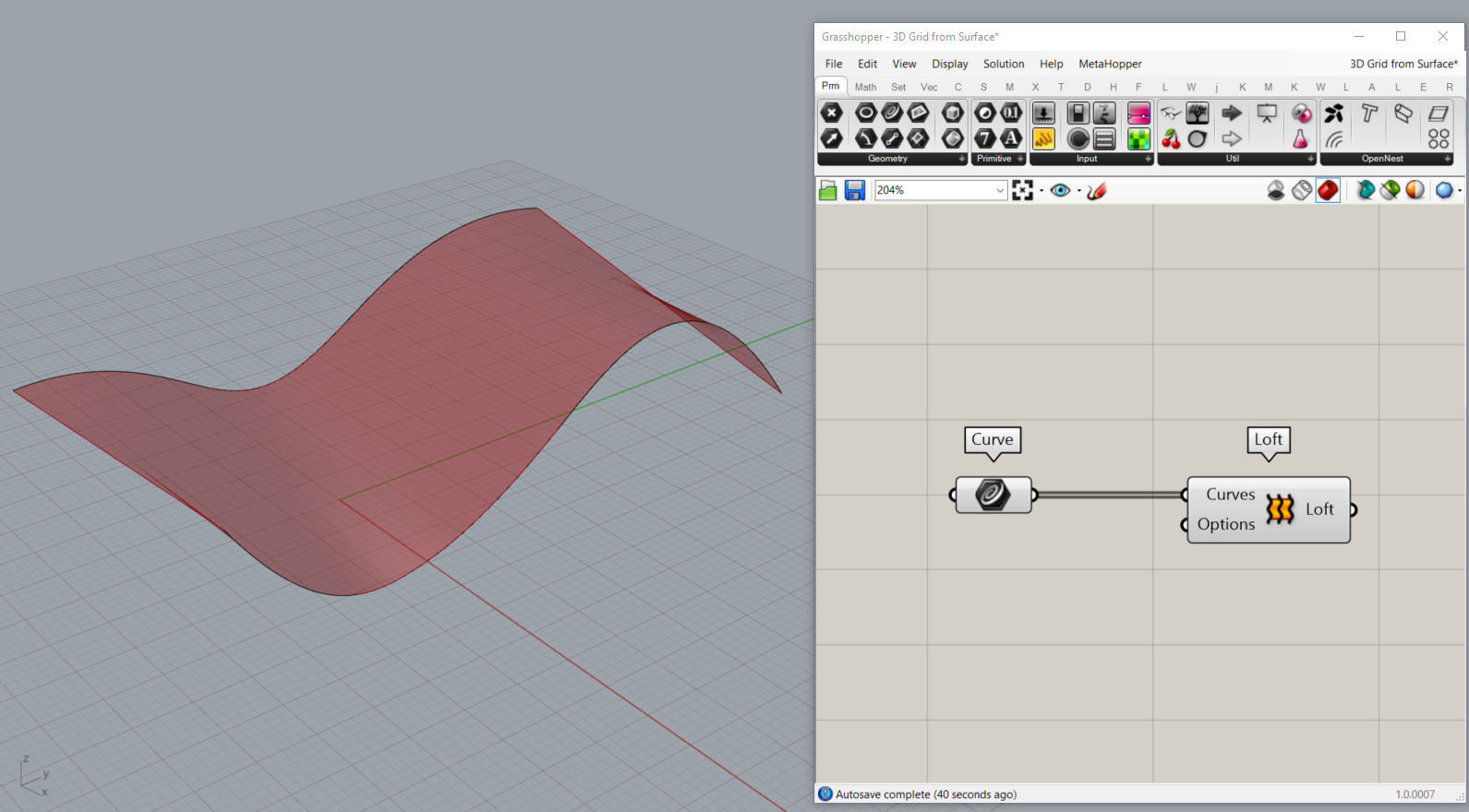
First you set two curves drawn in Rhino and create a loft between them using the loft component.
- Create two curves in Rhino
- Create a curve parameter in Grasshopper
- Set the curves on the curve parameter
- Loft the curves
Subdivide the surface with UV segments using the isotrim component. The result is a series of smaller surfaces, in other words a panelized surface. These are the cells of your grid.
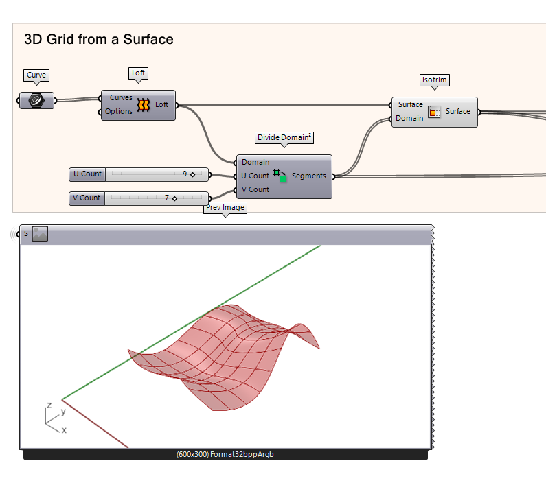
- Subdivide the surface
- Connect two number sliders to the U and V
- Trim the surface using the UV domain
3D Grid From Surface 2/5
BoxMorphlink copied
Once the surface is panelized into a uv-grid, you can use it for many different transformations. One of the transformations we will demonstrate here are the Surface Box and the BoxMorph tool. A SurfaceBox creates 3D cells (with a specified height) from the 2D cells of the divided Surface. The Boxmorph places an object within those 3D cells, automatically adjusting the dimensions of your geometry. It adjusts the BoundingBox of the geometry to match the 3d boxes on the surface and scales the geometry accordingly.
First, you need to convert the 2D cells to 3D by using the SurfaceBox command. Connect the original surface and use the Domain from the Divide Domain component. Specify the Height by using a Number Slider. Now you have generated the Target boxes for the geometry.
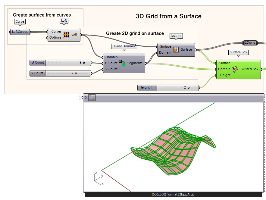
- Create boxes on the grid using the surface, isotrim and a Height number slider as input Create boxes on the grid using the surface, isotrim and a Height number slider as input
- Define the height with a Number Slider. You may have to use a negative value
Now you can create a geometry in Rhino that you want to morph over the surface. Then set it on a geometry parameter in Grasshopper.
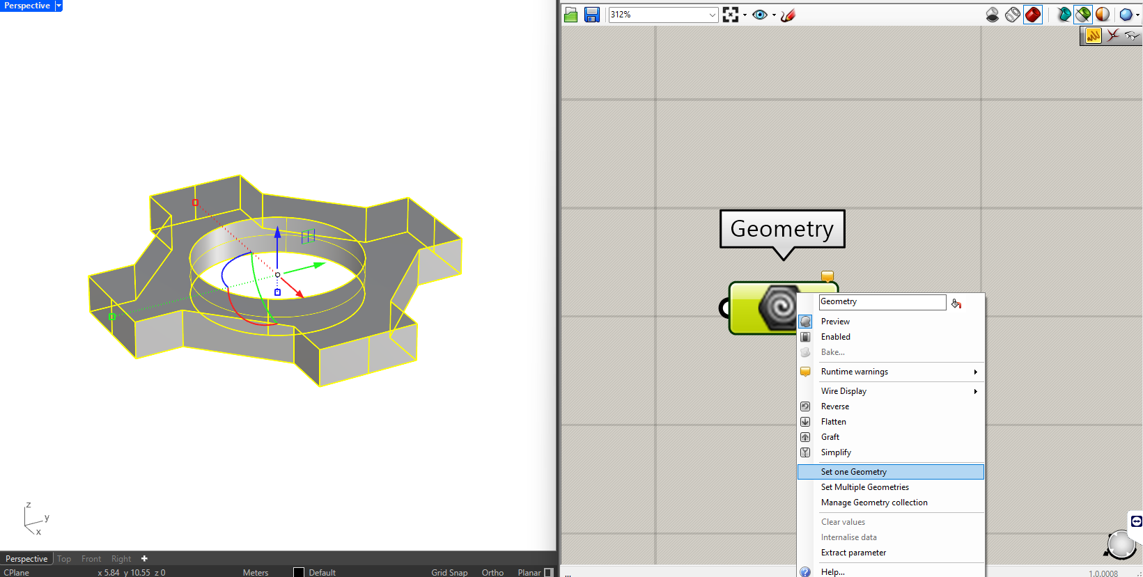
- Design the geometry you want to morph over the surface in Rhino
- Create a geometry parameter
- Set the geometry on the parameter
Now we create a bounding box around the object. A bounding box is the smallest possible box around an object using the axes of a specific plane. After that, we morph the geometry back to the surface.
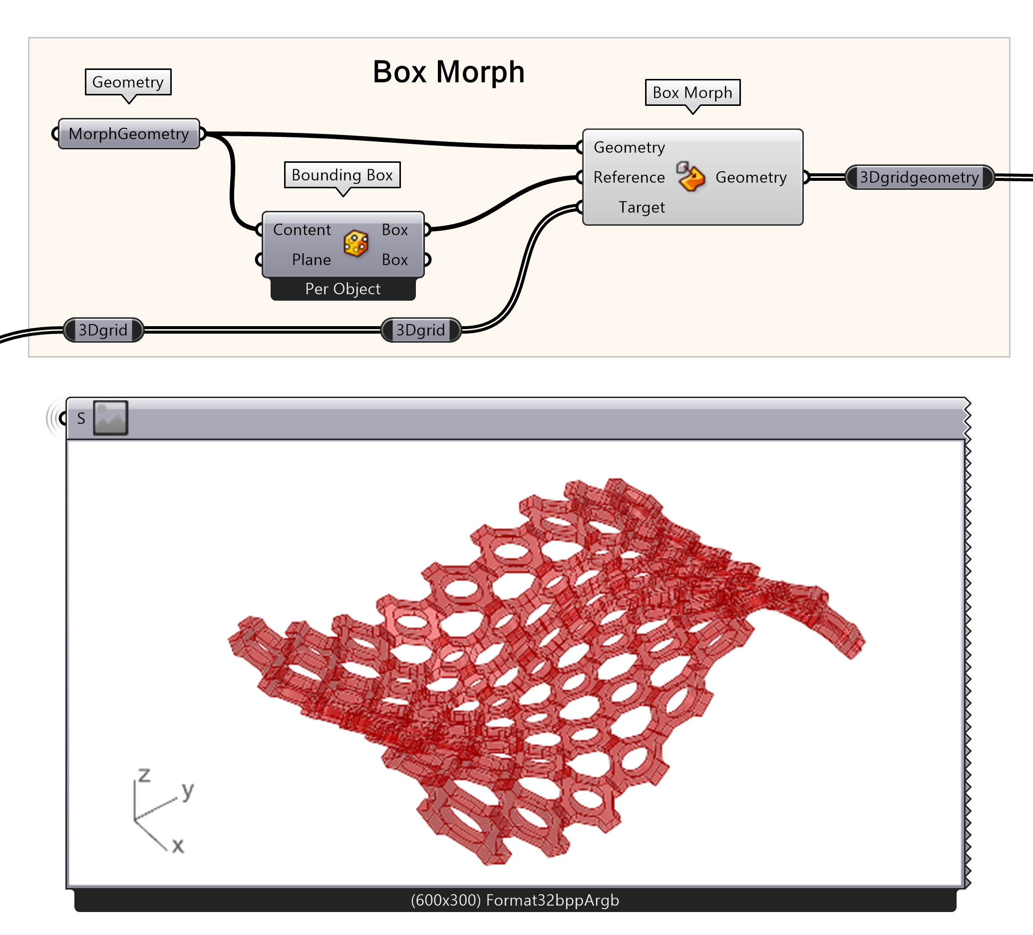
- Use the bounding box function on the geometry using the content input
- Create a surface morph node. Plug the BoundingBox into the Reference Box input on the Boxmorph tool. Finally add the Target boxes from the SurfaceBox command.
Note: The box morph is a computationally expensive process, so it may take a while to get the result.
If you want to morph multiple objects to the surface, you can change the bounding box setting by right-clicking and selecting Union Box. You also need to group the objects for the Geometry input.
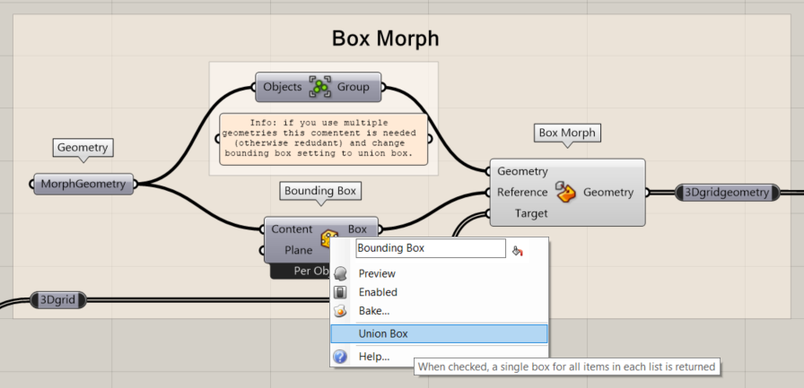
- If using multiple geometries, set bounding box to union box
- Group the geometries before the Geometry input
3D Grid From Surface 3/5
Surface Analysislink copied
The surface subdivision can also be useful in analyzing the surface. For example, by using Evaluate Surface node, we can evaluate the surface based on a uv coordinate. UV coordinates refer to the domain of the surface. For our purposes we will reparametrize the surface, meaning we redistribute the uv domain from 0-1.
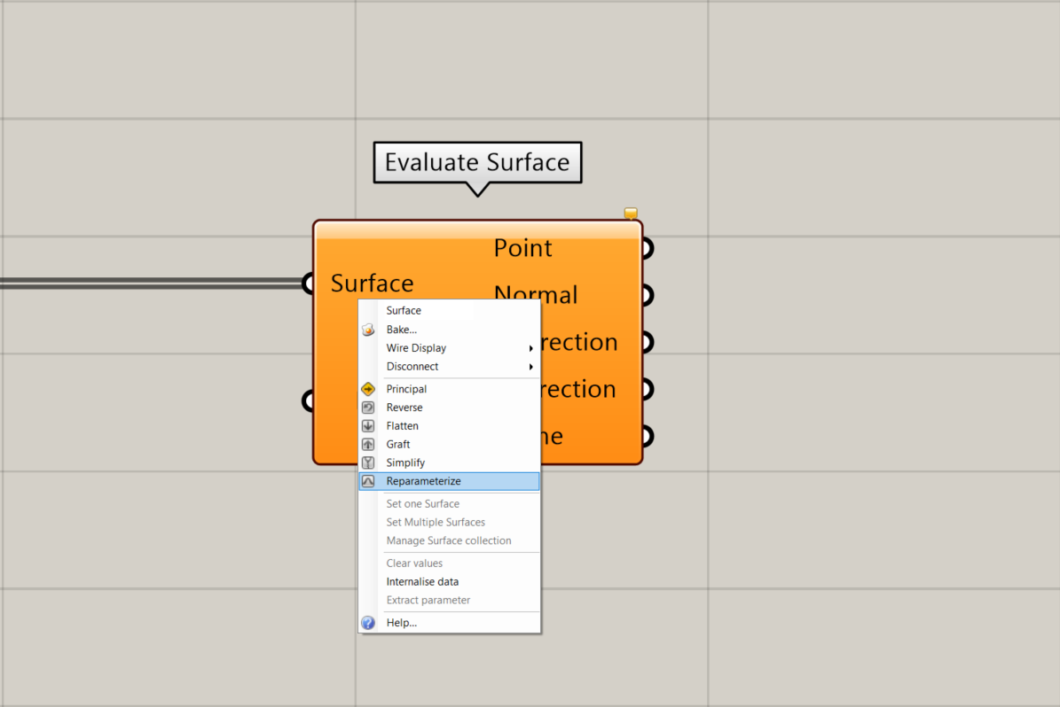
- Connect the isotrim surface to an Evaluate Surface node
- Right-click on the Surface input of the Evaluate Surface component and select Reparametrize
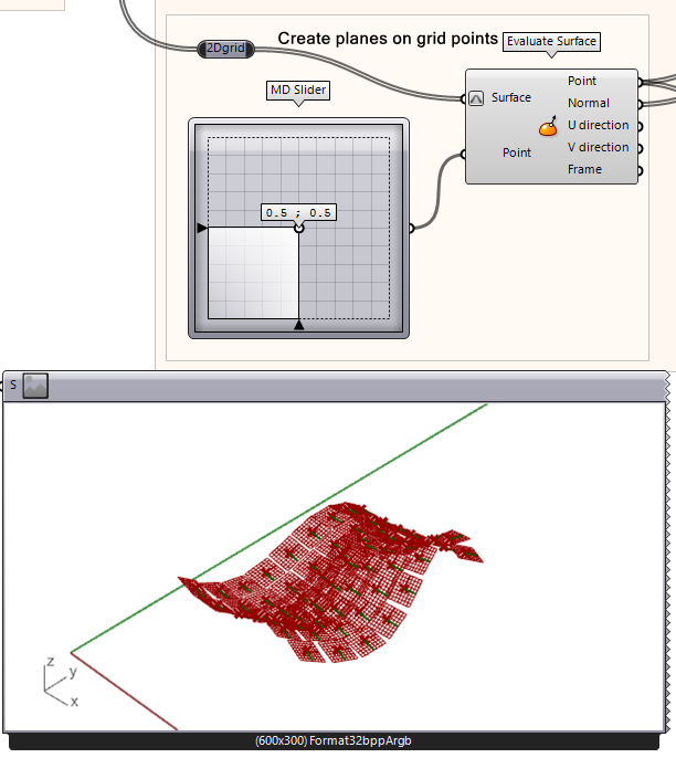
Using the MD Slider is visually easy to understand as the square lay-out of the slider mimics the uv-point in relation to the surface. The output of the slider is a x,y,z coordinate where the z is always 0.
§ Calculate the center point of the surface with the MD Slider, do not change the values
§ Connect the MD Slider output to the Point input of the Evaluate Surface node
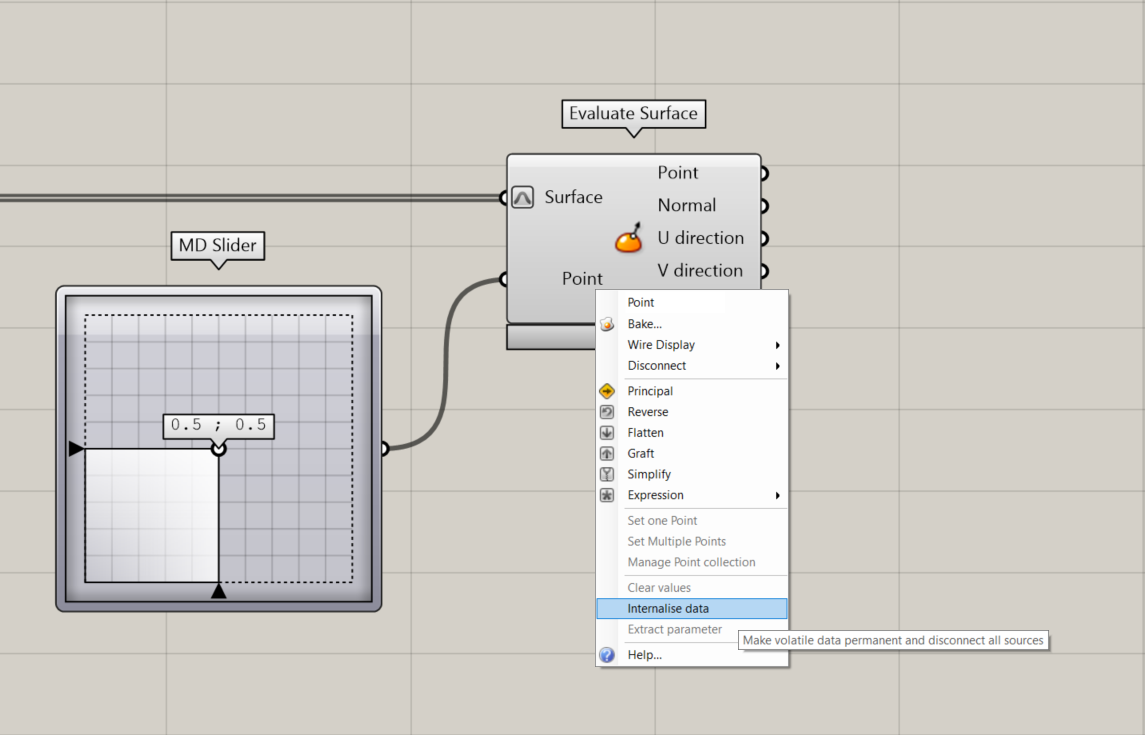
To keep your definition compact you can decide to internalize the uv-coordinate. This means that the data is stored inside the component and is permanent until substituted with another input. Right-click the uv-input and select internalize data.
3D Grid From Surface 4/5
Color by Slopelink copied
The Evaluate Surface component returns a Point, a Normal and a frame A plane derived from geometry (plane derived from geometry). We can use this data to analyze the curvature of the surface. In order to visualize this data, we will color the subdivisions according to their slope. This could be useful when you are generating a walkable surface and the slope cannot by higher than 10% (wheelchair accessibility, for example. This can be done in many ways, but to understand the process exactly we calculate the vector of the normal compared to a vertical vector. If we multiply this by 100, we obtain the slope percentage.
To visualize the process, we will first draw two SDL-lines. One SDL-line will Start from the evaluated surface Point following the Direction of the Normal. The Length doesn’t matter, a Number Slider can be used in this case. The other SDL-line follows the z-Direction, Starting from the same Point, using the same Number Slider for the Length. Make sure they have the same orientation, if not (like in the example here) one of them needs to be inverted by using the negative component.
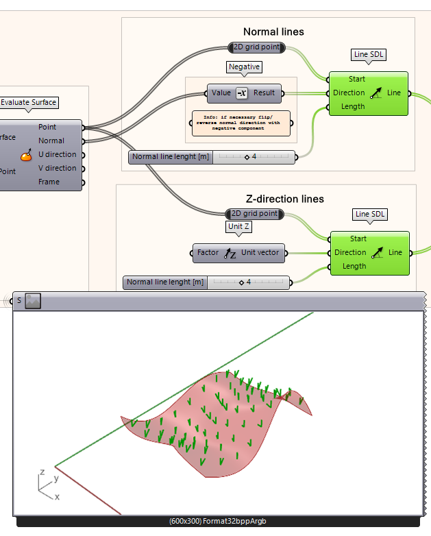
- Create two SDL-lines from the Evaluate Surface Point output
- Define a random length with a Number Slider
- For the first SDL connect the output Normal from the Evaluate Surface component.
- If necessary, flip the direction of one of the SDL line direction inputs
- For the second SDL line use a Z-Unit Vector as input,
Now we extract the Endpoints of the lines to easily generate a 2-Point Vector, ensuring the correct direction of both vectors instantly.
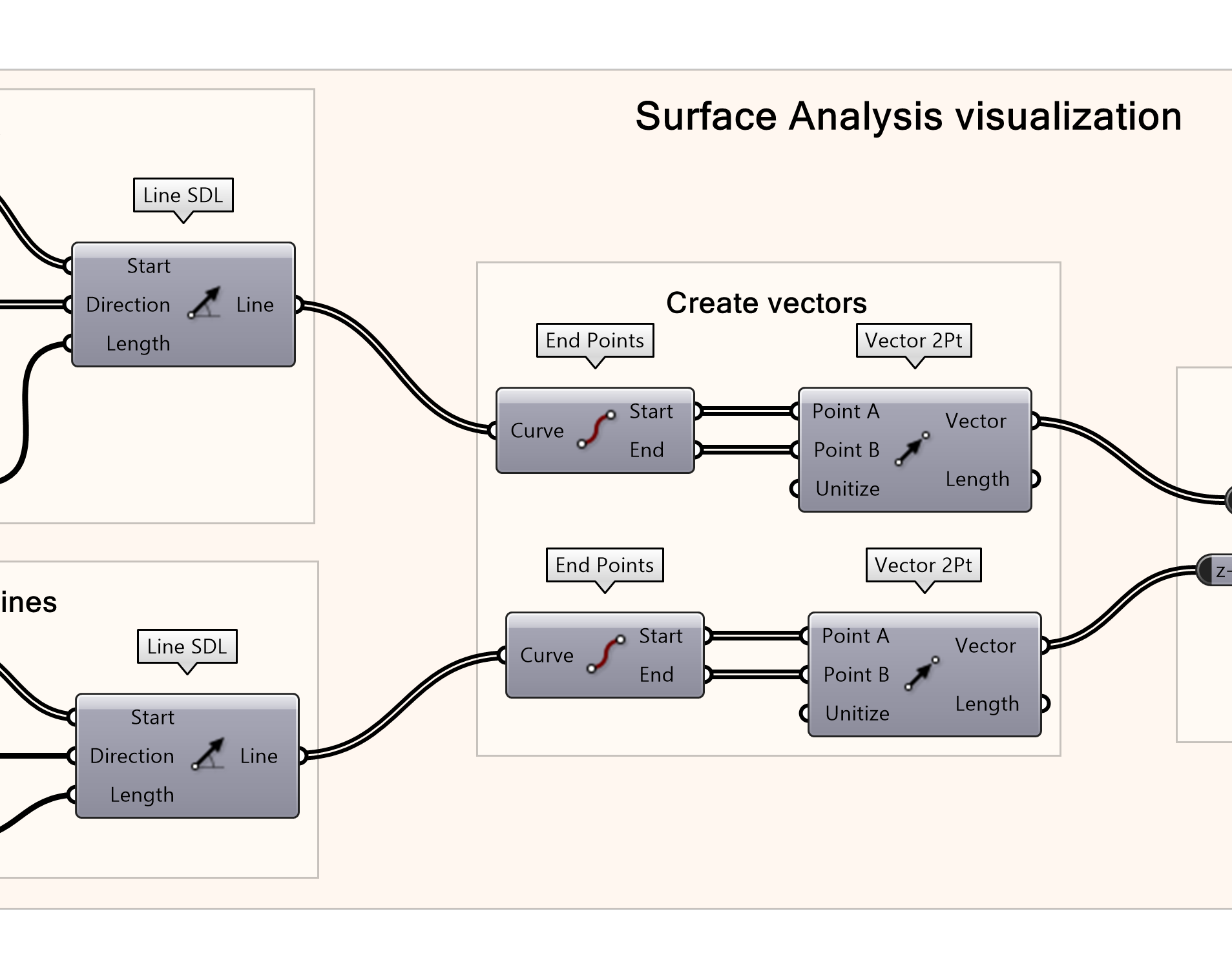
- Find the endpoints of the SDL lines
- Create two vectors from the endpoints per line
Compute the angle between the two vectors. This equals the slope since calculating the difference between the horizontal vector and the tangent vector on the surface (90 degrees rotated normal) returns the same number.
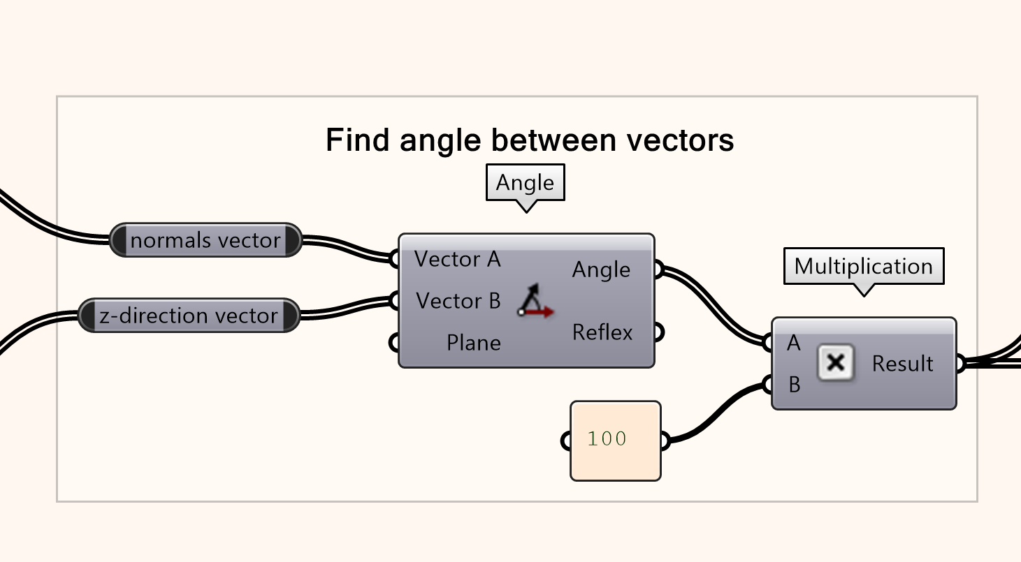
- Compute the angle between the vectors
- Multiply the output angle with 100 by adding a number slider or a panel with the value 100. Or right-clicking on input ‘B’, hovering over ‘Set Data Item’, enter the number then ‘Commit Changes.’
The final visualization of our model requires an upper limit of the color gradient. We can use the highest angle from the surface geometry as our upper limit. To do so use, a Sort List component and reverse the outcome keys. The use a list item to select the highest value in the list.
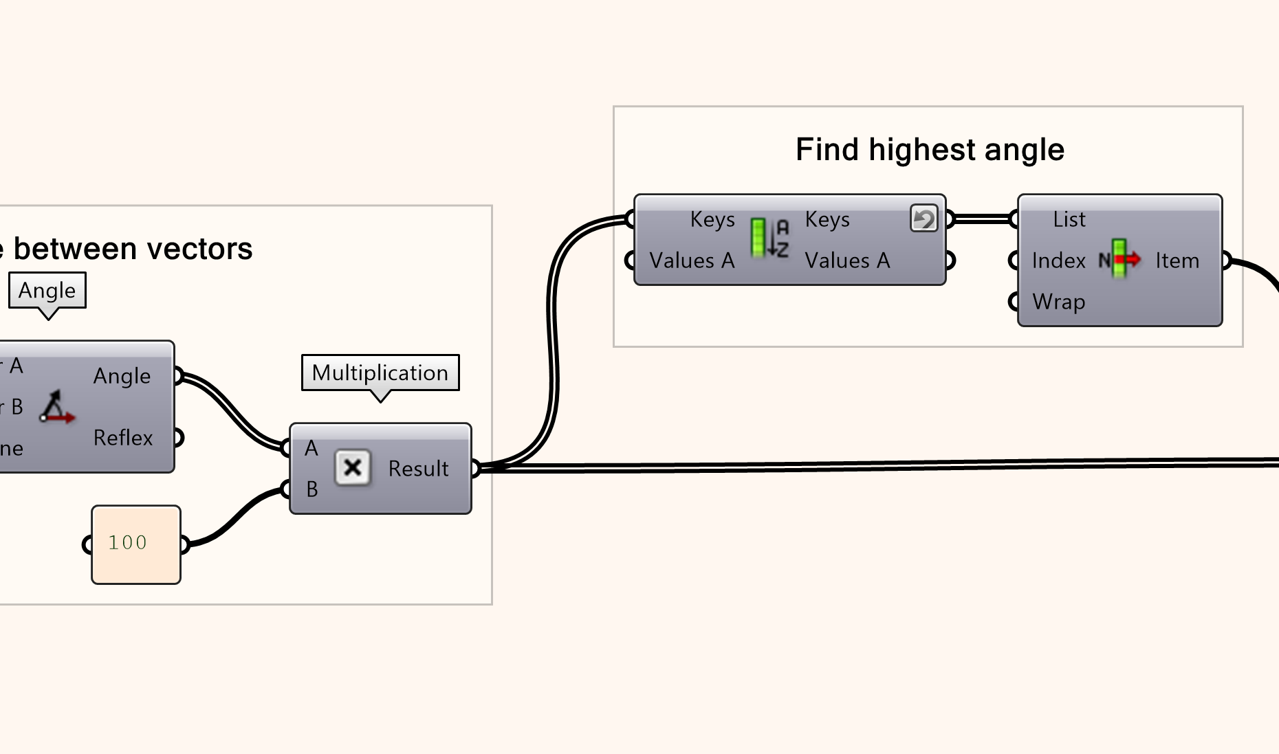
- Find the highest value by using the following, then right-click on keys and select ‘Reverse’.
- Select the first item using the following. That Bullet points with component location.
For a colored representation of the different slopes we can use a color gradient option. Connect the slope percentages from the Multiplication component into the Parameter t of the Color Gradient. Plug the Divided Surface geometry into a Custom Preview component. Then enter the output of the Color Gradient into the Color input of the Custom Preview.
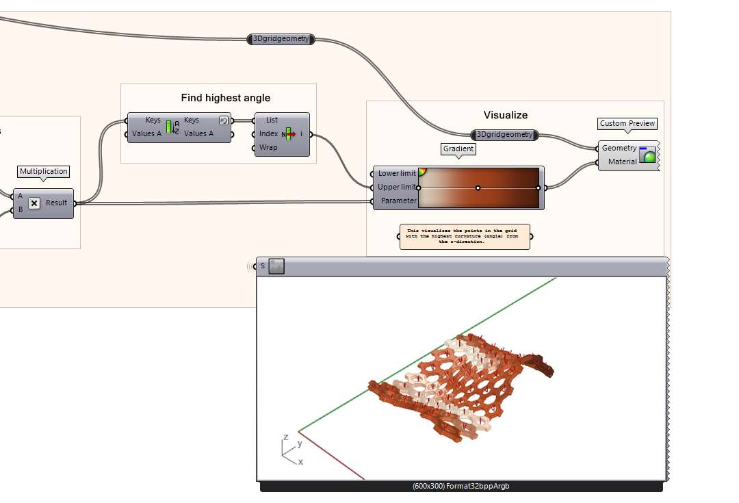
- Display the angles of the surface using the t input of a gradient
- The highest angle output will be your input for the upper-limit input of the Gradient component.
- Connect the gradient output to a Custom Preview Shader input
- Connect the isotrim surfaces to the geometry input of the Custom Preview node
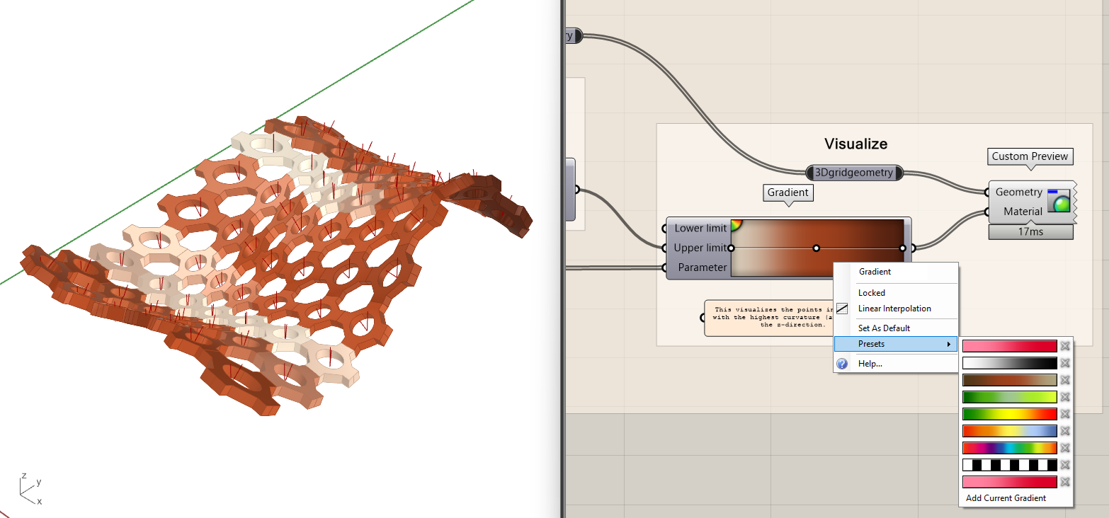
There are different pre-sets if you right-click on the colored component. Moving the small dots adjusts the corresponding colors and percentages.
3D Grid From Surface 5/5
Conclusionlink copied
In conclusion, you learned how to create a 3D grid using a freeform surface as the basis for the grid, and populate the grid with a defined geometry, and morph it into the surface to create a 3-dimensional geometry. Additionally, you learned how to analyze a surface based on their angles and visualize them using custom gradient presets.

Write your feedback.
Write your feedback on "3D Grid From Surface"".
If you're providing a specific feedback to a part of the chapter, mention which part (text, image, or video) that you have specific feedback for."Thank your for your feedback.
Your feedback has been submitted successfully and is now awaiting review. We appreciate your input and will ensure it aligns with our guidelines before it’s published.
