Predicting Room Labels
-
Intro
-
Design and Files
-
Video: Predicting Room Labels with Three Different ML Models
-
Loading the dataset
-
Data Visualization
-
Training Preparation
-
K-Nearest Neighbors
-
Random Forest
-
Neural Networks
-
Comparing ML Models
-
Testing ML Models with Additional Data
-
Conclusion
Information
| Primary software used | Jupyter Notebook |
| Course | Computational Intelligence for Integrated Design |
| Primary subject | AI & ML |
| Secondary subject | Machine Learning |
| Level | Intermediate |
| Last updated | November 27, 2024 |
| Keywords |
Responsible
| Teachers | |
| Faculty |
Predicting Room Labels 0/11
Predicting Room Labels
This tutorial will guide you through using three different machine learning methods to predict room labels for rooms in a generated data set. This will be done using python in a Jupyter notebook. The ML methods used are K-Nearest Neighbors, Decision Trees, and a Neural Network.
In an earlier tutorial, we created a parametric model is put together in grasshopper to gather data about the daylight, glare, and room features which are exported into excel, as seen in
In this tutorial, we will import the data from a CSV file into a Jupyter notebook and use this data to train three different machine learning models. Based on the best performing model, we will export the predicted labels back to excel.
For this tutorial you need to have installed Python, Jupyter notebooks, and some common libraries including Scikit Learn. Please see the following tutorial for more information.
Predicting Room Labels 1/11
Design and Fileslink copied
This example refers to design overview described in
The university has described that they have a series of rooms that are a variable depth. Each room has a window on the shorter south side, which varies in width and height, and additionally, some rooms have shading. We need to predict what function each room should have based on the characteristics of the room.
Tutorial Files
Use the data set generated in the “Generating a Dataset in Grasshopper” tutorial. This file is also provided here.
The Jupyter notebook file can be downloaded here.
Predicting Room Labels 2/11
Video: Predicting Room Labels with Three Different ML Modelslink copied
Predicting Room Labels 3/11
Loading the datasetlink copied
The first step is to load the dataset into the Jupyter notebook. The CSV file is loaded in the Jupyter notebook and the values are stored in a dataframe.
Start by importing the python libraries of tabulate and pandas.’ In the variable “folder” replace the noted file path with the location of where you stored the downloaded file. Ensure that if it is in a .zip folder, you first unzip it. Also ensure you use forward slashes in the file path. If you renamed the file name in the file_location variable must also be updated.
In line 12, we create a dataframe from the CSV file.
In lines 15-22, we clean up the CSV file by removing unnecessary columns, adding a column to save the room number, and saving the modified CSV file.
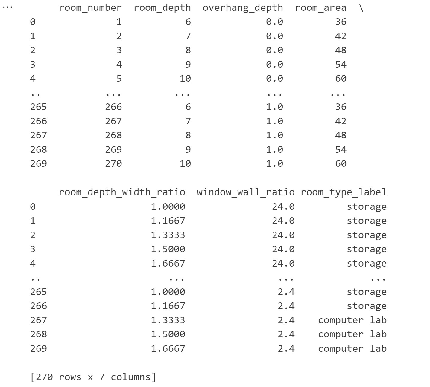
In lines 25-30 we load this modified CSV file into a dataframe and drop the columns with data that are not needed for training. For this example exercise we will train the model only with the width-depth ratio, the window-wall ratio and the overhang depth of the rooms, so the columns that are not needed are the window dimensions.
from tabulate import tabulate
import pandas as pd

#update this location to indicate where you have placed your files. Enter it as a string and make sure to use forward slashes (/)
folder = 'C:/Users/USER/Desktop/'
file_location = folder + '/data.csv'
save_file_location = folder + '/room_features_with_predictions_test.csv'

import pandas as pd

# Put the csv data in a dataframe
df = pd.read_csv(file_location)

# Remove 'in:' and 'out:' from the column names
df.columns = df.columns.str.replace(r'^(in:|out:)', '', regex=True)

# Add the room_number column at the beginning
df.insert(0, 'room_number', range(1, len(df) + 1))

# Save the modified DataFrame to a new CSV file
modified_csv_file =  folder + 'output.csv'
df.to_csv(modified_csv_file, index=False)


df_loaded = pd.read_csv(modified_csv_file, sep=",", header=0)
df_csv = df_loaded
#remove excess columns that are not relevant for training

#remember for this problem, we will only train on the WidthDepthRatio, WindowWallRatio, and ShadingDepth features of the room
df = df_loaded.drop(["window_width","window_height", "name", "DA_median", "UDI_median", "UDI_low_median", "UDI_up_median", "img_1", "img_2"], axis=1)
#! don't forget to only load the data we need, remove the extra columns that save the width, etc

#visualzing the loaded data
#print(tabulate(df, headers='keys', tablefmt='psql'))
print(df)
Predicting Room Labels 4/11
Data Visualizationlink copied
Before we train the model, it is important to visualize the data set to understand some of the relationships that may exist in the data. First, we count how many rooms exist in the dataset per type and get their percentage in regard to the sum of the room variations. Run the cell to get the results. We can see that the data set contains 270 rooms total with 63 computer labs, 107 storage rooms, and 100 offices. Of the total rooms 23.0% are computer labs, 40.0% are storage rooms, and 37.0% are offices.
cl_count = (df['room_type_label'] == "computer lab").sum()
storage_count = (df['room_type_label'] == "storage").sum()
office_count = (df['room_type_label'] == "office").sum()

cl_percent = round(cl_count/len(df['room_type_label']), 2)*100
storage_percent = round(storage_count/len(df['room_type_label']), 2)*100
office_percent = round(office_count/len(df['room_type_label']), 2)*100

print('The data set contains {} rooms total with {} computer labs, {} storage rooms, and {} offices'.format(len(df['room_type_label']), cl_count, storage_count, office_count))
print('Of the total rooms {}% are computer labs, {}% are storage rooms, and {}% are offices'.format(cl_percent, storage_percent, office_percent))

Next, we format the data to be able to visualize different features in a graph. Import the numpy, matplotlib.pyplot libraries and the module of ‘LabelEncoder’ from the sklearn.preprocessing library. Before plotting the graphs we assign the data to variables in lines 6 to 9 and encode the class labels based on the room type in lines 13 to 16.
The data assignment part of the script assigns specific columns from the DataFrame (df) to new variables for easier access and manipulation. The encoding part encodes the categorical labels in the ‘room_label’ column into numeric labels (‘classes_vis’), making them suitable for machine learning tasks. The Scikit LabelEncoder class automatically selects classes in alphabetical order so for our case, Class 0: Computer Lab, Class 1: Office, Class 2: Storage.
import numpy as np
import matplotlib.pyplot as plt
from sklearn.preprocessing import LabelEncoder

#assign data to variables
area_vis = df.loc[:, "room_area"]
wdratio_vis = df.loc[:, "room_depth_width_ratio"]
wwratio_vis = df.loc[:, "window_wall_ratio"]
shading_vis = df.loc[:, "overhang_depth"]

#encode class labels
#Class 0: Computer Lab; Class 1: Office; Class 2: Storage
classes_all = df.loc[:, "room_type_label"]
le = LabelEncoder()
le.fit(classes_all)
classes_vis = le.transform(classes_all)
Window to Wall Ratio and Area Graph
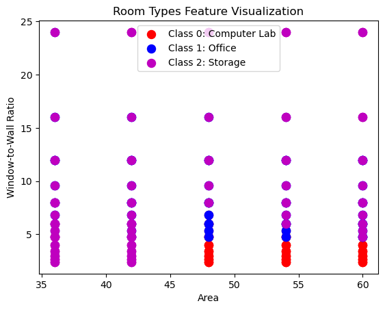
In the first graph, we will visualize the relationship between the window to wall ratio and the area based on the three classes.
To do this we first zip together the x axis (the room area) and y axis (the window to wall ratio). Then we separate the X, Y values into three separate lists, one for each class in lines 5 to 7. Finally, we create our visualization visualizing each class separately and assigning a different color.
# plot area and window-wall ratio
features_vis = list(zip(area_vis, wwratio_vis))

# plot the records here
class_0 = np.array([w[0] for w in zip(features_vis, classes_vis) if w[1] == 0])
class_1 = np.array([w[0] for w in zip(features_vis, classes_vis) if w[1] == 1])
class_2 = np.array([w[0] for w in zip(features_vis, classes_vis) if w[1] == 2])

plt.scatter(class_0[:, 0], class_0[:, 1], s=75, c='r', label = "Class 0: Computer Lab")
plt.scatter(class_1[:, 0], class_1[:, 1], s=75, c='b', label = "Class 1: Office")
plt.scatter(class_2[:, 0], class_2[:, 1], s=75, c='m', label = "Class 2: Storage")
plt.title('Room Types Feature Visualization')
plt.xlabel('Area')
plt.ylabel('Window-to-Wall Ratio')
plt.legend()
plt.show()
Window to Wall Ratio and Depth to Width Ratio Graph
We repeat the same process but this time for the window to wall ratio and the width to depth ratio. The visualization again visualizes each class in a different color.
# plot width-to-depth ratio and window-to-wall ratio
features2_vis = list(zip(wdratio_vis, wwratio_vis))

# plot the records here
class_0 = np.array([w[0] for w in zip(features2_vis, classes_vis) if w[1] == 0])
class_1 = np.array([w[0] for w in zip(features2_vis, classes_vis) if w[1] == 1])
class_2 = np.array([w[0] for w in zip(features2_vis, classes_vis) if w[1] == 2])

plt.scatter(class_0[:, 0], class_0[:, 1], s=75, c='r', label = "Class 0: Computer Lab")
plt.scatter(class_1[:, 0], class_1[:, 1], s=75, c='b', label = "Class 1: Office")
plt.scatter(class_2[:, 0], class_2[:, 1], s=75, c='m', label = "Class 2: Storage")
plt.title('Room Types Feature Visualization')
plt.xlabel('Width-to-Depth Ratio')
plt.ylabel('Window-to-Wall Ratio')
plt.legend()
plt.show()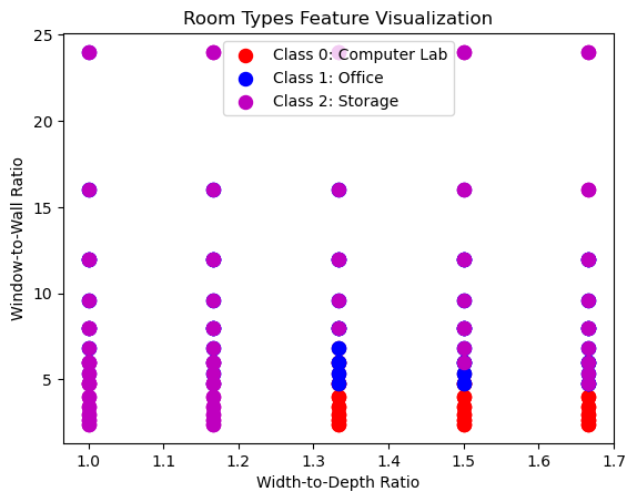
Predicting Room Labels 5/11
Training Preparationlink copied
To train our model, we must first encode our class labels. Then we can normalize the data, split it into training and test sets, and finally train the three different models.
We start by encoding all data into labels. First, the script extracts the ‘room_label’ column from the DataFrame. We then use the LabelEncoder to fit and transform these labels into numeric format. Finally, in Line 8 we replaces the original ‘room_label’ column in the DataFrame with these numeric labels.
#encode class labels
#Class 0: Computer Lab; Class 1: Office; Class 2: Storage
classes_all = df.loc[:, 'room_type_label']
le = LabelEncoder()
le.fit(classes_all)
classes = le.transform(classes_all)

df['room_type_label'] = classes
Import the necessary modules of ‘train_test_split’, ‘make_pipeline’, ‘Pipeline’, ‘StandardScaler’, ‘LogisticRegression’ from the scikit-learn library for model training and preprocessing.
Our dataframe contains all the characteristics of the rooms including the class label which the model will predict. Therefore we need to split the data frame and assign it to different variables.
The model will train on the room features which will be the variable X. This requires dropping the “room_type_label” column as shown in line 7. In line 8, we assign the “room_type_label” column of the data frame as the target variable, which is y.
In Lines 12-20, the script scales the data by standardizing the features to ensure they have a mean of 0 and a standard deviation of 1 and then updates the DataFrame with the normalized values.
Finally, in line 23, the script splits the dataset into training and testing sets to evaluate the ML model. We use 70% of the data for training and 30% for testing.
from sklearn.model_selection import train_test_split
from sklearn.pipeline import make_pipeline
from sklearn.pipeline import Pipeline
from sklearn.preprocessing import StandardScaler
from sklearn.linear_model import LogisticRegression

X = df.drop(['room_type_label'], axis=1)
y = df.room_type_label
X_norm = X

# Normalize data
scaler = StandardScaler()
X_normalized = scaler.fit_transform(X)

for index, row in X_norm.iterrows():
    X_norm.at[index, 'room_area'] = X_normalized[index, 0]
    X_norm.at[index, 'room_depth'] = X_normalized[index, 1]
    X_norm.at[index, 'room_depth_width_ratio'] = X_normalized[index, 2]
    X_norm.at[index, 'window_wall_ratio'] = X_normalized[index, 3]
    X_norm.at[index, 'overhang_depth'] = X_normalized[index, 4]

# Split dataset into training set and test set
X_train, X_test, y_train, y_test = train_test_split(X_norm, y, test_size=0.3) # 70% training and 30% test
We are now ready to start training the model based on the 3 ML methods.
Predicting Room Labels 6/11
K-Nearest Neighborslink copied
This chapter uses K-Nearest Neighbors. If you need additional information on K-Nearest Neighbors, please see the relevant videos and notebook.
After importing the modules ‘make_classification’, ‘KNeighborsClassifier’ from the scikit-learn library. We first create the KNN classifier in line 6, train the model in line 9, and use it to predict the values of the test data set in line 12. The prediction is the encoded numerical value we encoded it to earlier. We can use the inverse_transform function to turn the numbers back into the room label strings.
The predicted values are zipped together with the row index so we can later save the predicted values back into the data frame. Line 20 and 21 prints the predicted values so we can see what they are.
# Load libraries
from sklearn.datasets import make_classification
from sklearn.neighbors import KNeighborsClassifier

#Create KNN Classifier
knn = KNeighborsClassifier(n_neighbors=5)

#Train the model using the training sets
knn.fit(X_train, y_train)

#Predict the response for test dataset
y_pred_KNN = knn.predict(X_test)
#Decode the predicted value back into the label
y_pred_KNN_string = le.inverse_transform(y_pred_KNN)

#Connect predicted values back to indexes to save in the proper place in the CSV
indexes = X_test.index.values
value_KNN = list(zip(indexes, y_pred_KNN_string))

print(y_pred_KNN)
print(y_pred_KNN_string)

Next, we need to save the predicted values back to a CSV file. To do this, we will import the csv library, add the predicted values back into the data frame and save the data frame to a CSV.
import csv

#add predicted label back to CSV and save to original excel file
df['knn_pred'] = np.nan
for pred in value_KNN:
    df.loc[pred[0], 'knn_pred'] = pred[1]

df_csv['knn_pred'] = df['knn_pred']

df_csv.to_csv(save_file_location, sep=",")
Finally, we can review the accuracy and the confusion matrix. A confusion matrix shows the predicted label along the X axis and the actual label along the Y axis. Therefore, all values in the diagonal starting with the top left and going down to the bottom right are the correct predicted labels. First, load the module of ‘metrics’ from the scikit-learn library for an accuracy calculation. The accuracy of the K-Nearest Neighbours classifier is 0.5925 this is not a very good accuracy and means that we need to adjust the hyperparameters or get better data to improve the accuracy of the model.
From the confusion matrix, we can see that the classifier frequently mis-classifies the storage spaces as either office or computer lab spaces.
#Import scikit-learn metrics module for accuracy calculation
from sklearn import metrics
# Model Accuracy, how often is the classifier correct?
print("Accuracy:",metrics.accuracy_score(y_test, y_pred_KNN))

# Which classes are commonly misclassified?
print('Confusion Matrix')
print(metrics.confusion_matrix(y_test, y_pred_KNN, labels=[0, 1, 2]))

#Save the information to variables to compare later
KNN_accuracy = metrics.accuracy_score(y_test, y_pred_KNN)
KNN_confusion = metrics.confusion_matrix(y_test, y_pred_KNN, labels=[0, 1, 2])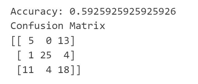
Predicting Room Labels 7/11
Random Forestlink copied
This chapter uses Random Forest. If you need additional information on Random Forest, please see the relevant videos and notebook.
We will now also train an Random Forest classifier to compare its performance to the other models. First load the required modules of ‘DecisionTreeClassifier’, ‘train_test_split’, ‘metrics’, ‘RandomForestClassifier’, ‘make_classification’ from the scikit-learn library.
# Load libraries
from sklearn.tree import DecisionTreeClassifier # Import Decision Tree Classifier
from sklearn.model_selection import train_test_split # Import train_test_split function
from sklearn import metrics #Import scikit-learn metrics module for accuracy calculation
from sklearn.ensemble import RandomForestClassifier
from sklearn.datasets import make_classification
Set Max Depth
For the Random Forest Classifier, it is possible to set the max_depth parameter which allows control over the size of the tree to prevent overfitting. You can see the impact of changing the max_depth parameter the relative misclassification cost against the maximum depth. The misclassification rate is calculated by taking the number of incorrect predictions and dividing these by the total number of predictions. The plot below shows which max_depth value is optimal.
from matplotlib import pyplot as plt

depth = []
accuracy = []

for i in range(1, 10):
    # Create Decision Tree classifer object
    clf = DecisionTreeClassifier(max_depth=i)
    # Train Decision Tree Classifer
    clf = clf.fit(X_train,y_train)
    #Predict the response for test dataset append accuracy for plotting
    y_pred_dt_vis = clf.predict(X_test)
    depth.append(i)
    accuracy.append(1 - metrics.accuracy_score(y_test, y_pred_dt_vis))

plt.plot(depth, accuracy, '-o')
plt.title('Misclassification vs Maximum Depth’)
plt.xlabel('Maximum Depth')
plt.ylabel('Relative Misclassification Cost')
plt.show()
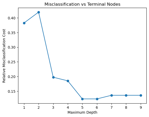
Based on the graph, we can see that the optimal maximum depth where the Y value is the lowest, should be around 5, therefore we also need to make sure that the max depth in the next cell is set to this number.
Train Classifier
In the next cell, the code creates and trains a Random Forest classifier with the specified parameters in lines 2 and 3, predicts labels for a test dataset in Line 6, decodes the predicted values back into their original labels in line 8, and connects the predicted values back to their corresponding indexes for saving in a CSV file in lines11-12. When running the cell we can see the predicted values printed below.
# Train Random Forest Classifer object with the correct max_depth value
clf = RandomForestClassifier(max_depth=5, random_state=0, n_estimators=50)
clf.fit(X_train,y_train)

#Predict the response for test dataset
y_pred_RF = clf.predict(X_test)
#Decode the predicted value back into the label
y_pred_RF_string = le.inverse_transform(y_pred_RF)

#Connect predicted values back to indexes to save in the proper place in the CSV
indexes = X_test.index.values
value_RF = list(zip(indexes, y_pred_RF_string))

print(y_pred_RF)
print(y_pred_RF_string)

Next, we need to save the predicted values back to a CSV file. To do this, we will add the predicted values back into the data frame and save the data frame to a CSV similarly to the way we did before with the KNN predicted values.
import csv

#add predicted label back to CSV and save to original excel file
df['rf_pred'] = np.nan
for pred in value_RF:
    df.loc[pred[0], 'rf_pred'] = pred[1]

df_csv['rf_pred'] = df['rf_pred']

df_csv.to_csv(save_file_location, sep=",")
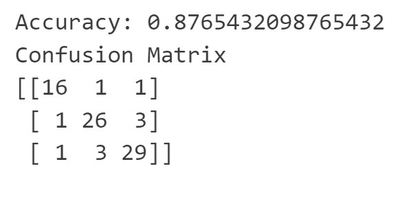
Finally, we can review the accuracy and the confusion matrix. The accuracy of the Random Forest classifier is 0.8765. We can see from the confusion matrix that there are few rooms which is predicted incorrectly. It has a tendency to confuse the office and storage rooms.
# Model Accuracy, how often is the classifier correct?
print("Accuracy:",metrics.accuracy_score(y_test, y_pred_RF))

# Which classes are commonly misclassified?
print('Confusion Matrix')
print(metrics.confusion_matrix(y_test, y_pred_RF, labels=None))

#Save the information to variables to compare later
RF_accuracy = metrics.accuracy_score(y_test, y_pred_RF)
RF_confusion = metrics.confusion_matrix(y_test, y_pred_RF, labels=[0, 1, 2])
Predicting Room Labels 8/11
Neural Networkslink copied
This chapter uses Neural Network. If you need additional information on Neural Networks, please see the relevant videos and notebook.
First load the required modules of ‘MLPClassifier’, ‘classification_report’, ‘metrics’, ‘confusion_matrix’, ‘accuracy_score’, ‘mean_squared_error’ from the scikit-learn library.
Then, create the Multi-Layer Perceptron (MLP) with 3 hidden layers that each contain 50 neurons in line 6, train the model in line 7, and use it to predict the values of the test data set in line 9.
Printed below the cell, we can see the predicted values.
#Load libraries
from sklearn.neural_network import MLPClassifier
from sklearn.metrics import classification_report,confusion_matrix
from sklearn.metrics import accuracy_score, mean_squared_error

mlp = MLPClassifier(hidden_layer_sizes = (50,50,50), random_state=1, max_iter=700)
mlp.fit(X_train, y_train)

y_pred_NN = mlp.predict(X_test)

#Decode the predicted value back into the label
y_pred_NN_string = le.inverse_transform(y_pred_NN)

#Connect predicted values back to indexes to save in the proper place in the CSV
indexes = X_test.index.values
value_NN = list(zip(indexes, y_pred_NN_string))
print(y_pred_NN)
print(y_pred_NN_string)

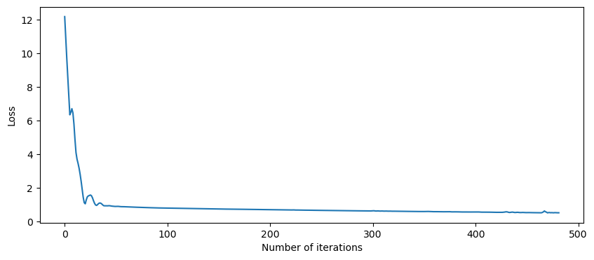
SciKit Learn tracks the loss curve along the training iterations. By plotting the loss against the iterations, it is possible to visualize if the model is learning. If the loss curve decreases first quickly, and then more slowly like the one below, the neural network is learning. If the loss curve jumps between high and low values or starts by decreasing and then jumps between high and low values, there may be problems with the model (for example, maybe the learning rate is too high) or with the data set (for example, too many outliers or noise in your data set). We can see from the loss-curve that the training is stable and converges.
import matplotlib.pyplot as plt

fig, ax = plt.subplots(figsize=(10,4))
ax.plot(mlp.loss_curve_)
ax.set_xlabel('Number of iterations')
ax.set_ylabel('Loss')
plt.show()
Evaluating Neural Networks
Precision
- Precision: is the number of true positive results divided by the total predicted positive values
- The total predicted positive values is the sum of the number of true positive results and the false positive results
- For multiple classes, it is the number of correctly classified samples of that class divided by the total number of samples that the classifier assigned to that class
Recall
- Recall: is the number of true positive results divided by the total number of positive results
- The total positive results is the sum of the number of true positive results and the false negative results
- For multiple classes, it is the number of correctly classified samples of that class divided by the total number of samples that actually belong to that class
F-score
- F-score is equal to two times the precision times the recall divided by the precision plus the recall
- F-score = 2 * (precision * recall) / (precision + recall)
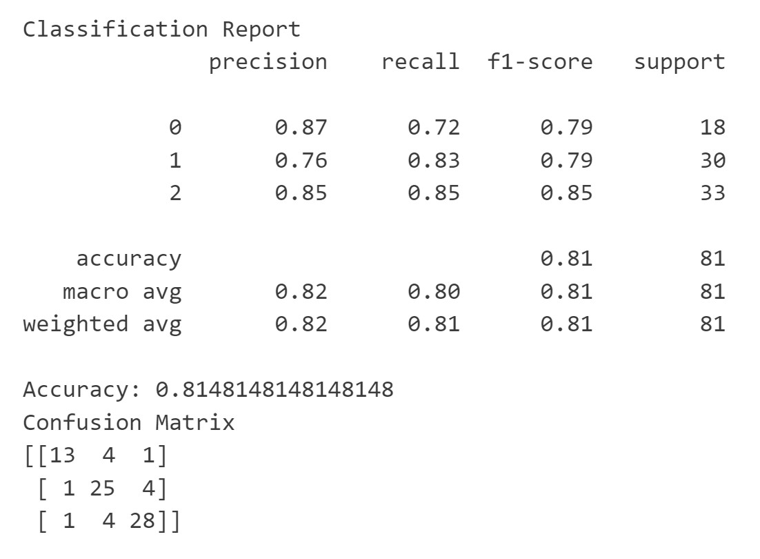
We can print these metrics by printing a classification report, accuracy score, and confusion matrix. We can see from the classification report that all the scores are fairly high, except that for class 1: offices, the MLP has a low precision predicting those. It is important to also look at the distribution of each class compared to the total number of rooms it is predicting. When looking at this, we can see that there are only 12 offices in our test data set so getting 1 wrong has a large impact therefore the percentages are lower than the other classes. In contrast, there are 44 storage rooms so getting 1 wrong has a smaller impact.
# Performance on testing dataset
print("Classification Report")
print(classification_report(y_test, y_pred_NN))
print("Accuracy:", accuracy_score(y_test, y_pred_NN))
print("Confusion Matrix")
print(confusion_matrix(y_test, y_pred_NN))

#Save the information to variables to compare later
NN_accuracy = accuracy_score(y_test, y_pred_NN)
NN_confusion = confusion_matrix(y_test, y_pred_NN)
Save to CSV
Next, we need to save the predicted values back to a CSV file. To do this, we will add the predicted values back into the data frame and save the data frame to a CSV.
import csv

#add predicted label back to CSV and save to original excel file
df['nn_pred'] = np.nan
for pred in value_RF:
    df.loc[pred[0], 'nn_pred'] = pred[1]

df_csv['nn_pred'] = df['nn_pred']

df_csv.to_csv(save_file_location, sep=",")
Predicting Room Labels 9/11
Comparing ML Modelslink copied

To compare the different models, we will visualize the confusion matrix for each method and look at the accuracy. To compare the three different options, please note that all models need to have been trained earlier in the notebook.
First we load the required libraries of numpy, matplotlib.pyplot, matplotlib.patheffects, seaborn, and pandas.
# Import libraries
import numpy as np
import matplotlib.pyplot as plt
import matplotlib.patheffects as path_effects
import seaborn as sns
import pandas as pd
By comparing the confusion matrix, it is possible to understand how each model performs for each class label. Each confusion matrix is displayed as a heatmap, with class labels along both axes. The diagonal elements represent the number of correctly classified instances for each class, while off-diagonal elements represent misclassifications. Text labels within each cell display the count of instances. The matrices are arranged side by side in a single plot for easy comparison, with titles indicating the classifier type. The plot is configured to show actual and predicted labels along the axes, enhancing interpretability.
data1 = KNN_confusion
data2 = RF_confusion
data3 = NN_confusion
class_names=[0,1,2] # name  of classes
tick_marks = np.arange(len(class_names))

# Basic Configuration
fig, (ax1, ax2, ax3) = plt.subplots(1, 3, figsize=(15, 5))

# Heat maps
im1 = ax1.imshow(data1, cmap="YlGnBu")
im2 = ax2.imshow(data2, cmap="YlGnBu")
im3 = ax3.imshow(data3, cmap="YlGnBu")

# Formatting for heat map 1
ax1.set_xticks(tick_marks)
ax1.set_yticks(tick_marks)
ax1.set_xticklabels(class_names)
ax1.set_yticklabels(class_names)
ax1.set_title('KNN Confusion Matrix', y=1.1)
ax1.xaxis.set_label_position("top")

# Formatting for heat map 2
ax2.set_xticks(tick_marks)
ax2.set_yticks(tick_marks)
ax2.set_xticklabels(class_names)
ax2.set_yticklabels(class_names)
ax2.set_title('RF Confusion Matrix', y=1.1)
ax2.xaxis.set_label_position("top")

# Formatting for heat map 3
ax3.set_xticks(tick_marks)
ax3.set_yticks(tick_marks)
ax3.set_xticklabels(class_names)
ax3.set_yticklabels(class_names)
ax3.set_title('NN Confusion Matrix', y=1.1)
ax3.xaxis.set_label_position("top")

# Graph Labels
ax1.set(xlabel='Predicted Label', ylabel='Actual Label')
ax2.set(xlabel='Predicted Label')
ax3.set(xlabel='Predicted Label')

# Text labels of each matrix
for i in range(len(class_names)):
    for j in range(len(class_names)):
        text = ax1.text(j, i, data1[i, j],
                       ha="center", va="center", color="black", fontweight="bold")
        text.set_path_effects([path_effects.Stroke(linewidth=3, foreground='white'),
                       path_effects.Normal()])

for i in range(len(class_names)):
    for j in range(len(class_names)):
        text = ax2.text(j, i, data2[i, j],
                       ha="center", va="center", color="black", fontweight="bold")
        text.set_path_effects([path_effects.Stroke(linewidth=3, foreground='white'),
                       path_effects.Normal()])

for i in range(len(class_names)):
    for j in range(len(class_names)):
        text = ax3.text(j, i, data3[i, j],
                       ha="center", va="center", color="black", fontweight="bold")
        text.set_path_effects([path_effects.Stroke(linewidth=3, foreground='white'),
                       path_effects.Normal()])

fig.tight_layout()
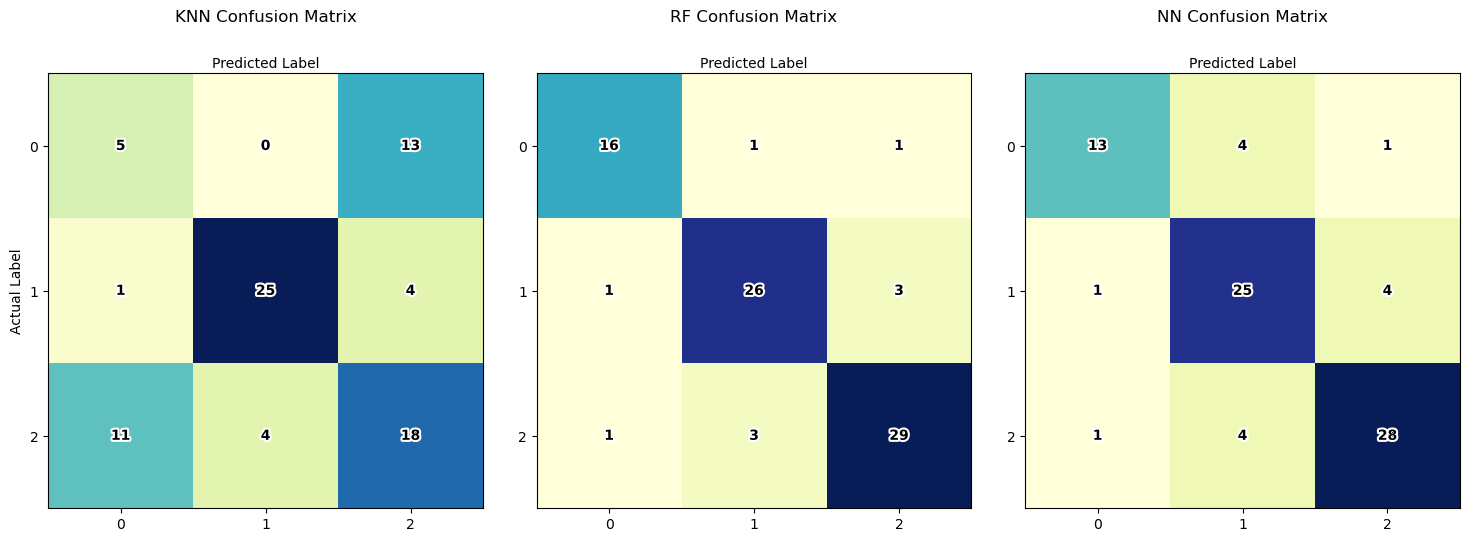
Based on the confusion matrix and the accuracy, we know that KNN did not perform very well as the accuracy was well below 80%. This can also be seen in the confusion matrix which has a lot of misclassifications. Random Forest and the Neural Network both did a fairly good job. We can see that for both models, the office and storage classes are frequently misclassified. This can tell us that we should add data that will help the model better distinguish these two classes.
Next we will print all of the accuracies so we can compare them. From this we can see that the Random Forest and Neural Network models are equally accurate, more accurate than the K-Nearest Neighbors model.
print('The data set contains {} rooms total with {} computer labs, {} storage rooms, and {} offices'.format(len(df['room_type_label']), cl_count, storage_count, office_count))
print('Of the total rooms {}% are computer labs, {}% are storage rooms, and {}% are offices'.format(cl_percent, storage_percent, office_percent))
print()
print("K-Nearest Neighbors Accuracy: ", round(KNN_accuracy, 2)*100, "%")
print("Random Forest Accuracy: ", round(RF_accuracy, 2)*100, "%")
print("Neural Network Accuracy: ", round(NN_accuracy, 2)*100, "%")

Predicting Room Labels 10/11
Testing ML Models with Additional Datalink copied
Start the video around 2:47 to follow along with the text.

The university has now received information about 10 new rooms. Let’s look at how we can use the trained models to predict the room labels for these rooms. The information provided by the university for the new rooms are written at the code in lists, added to the Dataframe and visualized in the following table.
#this is the data for the new rooms
np.random.seed(18)
num_rows = 10
room_numbers = ['room_1025', 'room_1313', 'room_1328', 'room_1400', 'room_1435', 'room_1436', 'room_1439', 'room_1570', 'room_1583', 'room_1612']

shading = [0,0.5,1]
wwr = [0.0417, 0.0625, 0.0833, 0.1042, 0.125, 0.1458, 0.1667, 0.1875, 0.2083, 0.25, 0.2917, 0.3333, 0.375, 0.4167]
width = 6
room_depths = np.random.randint(6, 10, size=num_rows)

areas = [i * width for i in room_depths]
depth_width_ratios = [i / width for i in room_depths]
window_wall_ratios = np.random.choice(wwr, size=num_rows)
shading_depths = np.random.choice(shading, size=num_rows)

new_rooms_df = pd.DataFrame({
    'room_number': room_numbers,
    'room_area': areas,
    'room_depth': room_depths,
    'room_depth_width_ratio': depth_width_ratios,
    'window_wall_ratio': window_wall_ratios,
    'overhang_depth': shading_depths
})

#visualzing the new data
print(tabulate(new_rooms_df, headers='keys', tablefmt='psql'))
When you have new data that you want to use with a model that was trained on normalized data, it’s important to apply the same scaling or normalization transformation to the new data. This ensures that the new data is consistent with the scale and distribution of the training data.
X_new = new_rooms_df.drop(['room_number'], axis=1)
X__new_norm = X_new

#normalize your data
X_new_normalized = scaler.transform(X_new)

for index, row in X__new_norm.iterrows():
    X__new_norm.at[index, 'room_area'] = X_new_normalized[index, 0]
    X__new_norm.at[index, 'room_depth'] = X_new_normalized[index, 1]
    X__new_norm.at[index, 'room_depth_width_ratio'] = X_new_normalized[index, 2]
    X__new_norm.at[index, 'window_wall_ratio'] = X_new_normalized[index, 3]
    X__new_norm.at[index, 'overhang_depth'] = X_new_normalized[index, 4]
After normalizing the data, we can use all three trained ML models to predict a room label for the new rooms.
#Using K-Nearest Neighbors
y_new_pred_KNN = knn.predict(X__new_norm)
#Decode the predicted value back into the label
y_new_pred_KNN_string = le.inverse_transform(y_new_pred_KNN)

#Using Random Forest
y_new_pred_RF = clf.predict(X__new_norm)
#Decode the predicted value back into the label
y_new_pred_RF_string = le.inverse_transform(y_new_pred_RF)

#Usng the Neural Network
y_new_pred_NN = mlp.predict(X__new_norm)
#Decode the predicted value back into the label
y_new_pred_NN_string = le.inverse_transform(y_new_pred_NN)

new_rooms_df['knn_pred'] = y_new_pred_KNN_string
new_rooms_df['rf_pred'] = y_new_pred_RF_string
new_rooms_df['nn_pred'] = y_new_pred_NN_string

#visualzing the new data with the room predictions
print(tabulate(new_rooms_df.drop(['room_area', 'room_depth', 'room_depth_width_ratio', 'window_wall_ratio', 'overhang_depth'], axis=1), headers='keys', tablefmt='psql'))

Predicting Room Labels 11/11
Conclusionlink copied
After following this tutorial you learned how to train 3 different machine learning models in Python using a Jupyter notebook. The three methods used were K-Nearest Neighbors, Random Forest and Neural Networks. Each model used the room features to learn what the expected room assignment (label) was of office, computer lab, and storage. The models trained to predict the label of the rooms and in the end, you applied it to new data.
Write your feedback.
Write your feedback on "Predicting Room Labels"".
If you're providing a specific feedback to a part of the chapter, mention which part (text, image, or video) that you have specific feedback for."Thank your for your feedback.
Your feedback has been submitted successfully and is now awaiting review. We appreciate your input and will ensure it aligns with our guidelines before it’s published.
