Gaussian Mixtures
-
Intro
-
Overview
-
Notebook
-
Conclusion
Information
| Primary software used | Jupyter Notebook |
| Course | Computational Intelligence for Integrated Design |
| Primary subject | AI & ML |
| Secondary subject | Machine Learning |
| Level | Intermediate |
| Last updated | November 11, 2024 |
| Keywords |
Responsible
| Teachers | |
| Faculty |
Gaussian Mixtures 0/3
Gaussian Mixtures
Gaussian Mixture Models (GMMs) are probabilistic models that assume data is generated from a mixture of several Gaussian distributions, each representing a cluster with its own mean and variance. GMMs are used for clustering by assigning probabilities for each data point belonging to each Gaussian component, allowing for soft assignment rather than hard clustering. Through the Expectation-Maximization (EM) algorithm, GMMs iteratively adjust the parameters of each Gaussian to best fit the data, effectively capturing the underlying distribution of complex datasets.
For this tutorial you need to have installed Python, Jupyter notebooks, and some common libraries including Scikit Learn. Please see the following tutorial for more information.

Download the Jupyter notebook here to follow along with the tutorial.
Gaussian Mixtures 1/3
Overviewlink copied
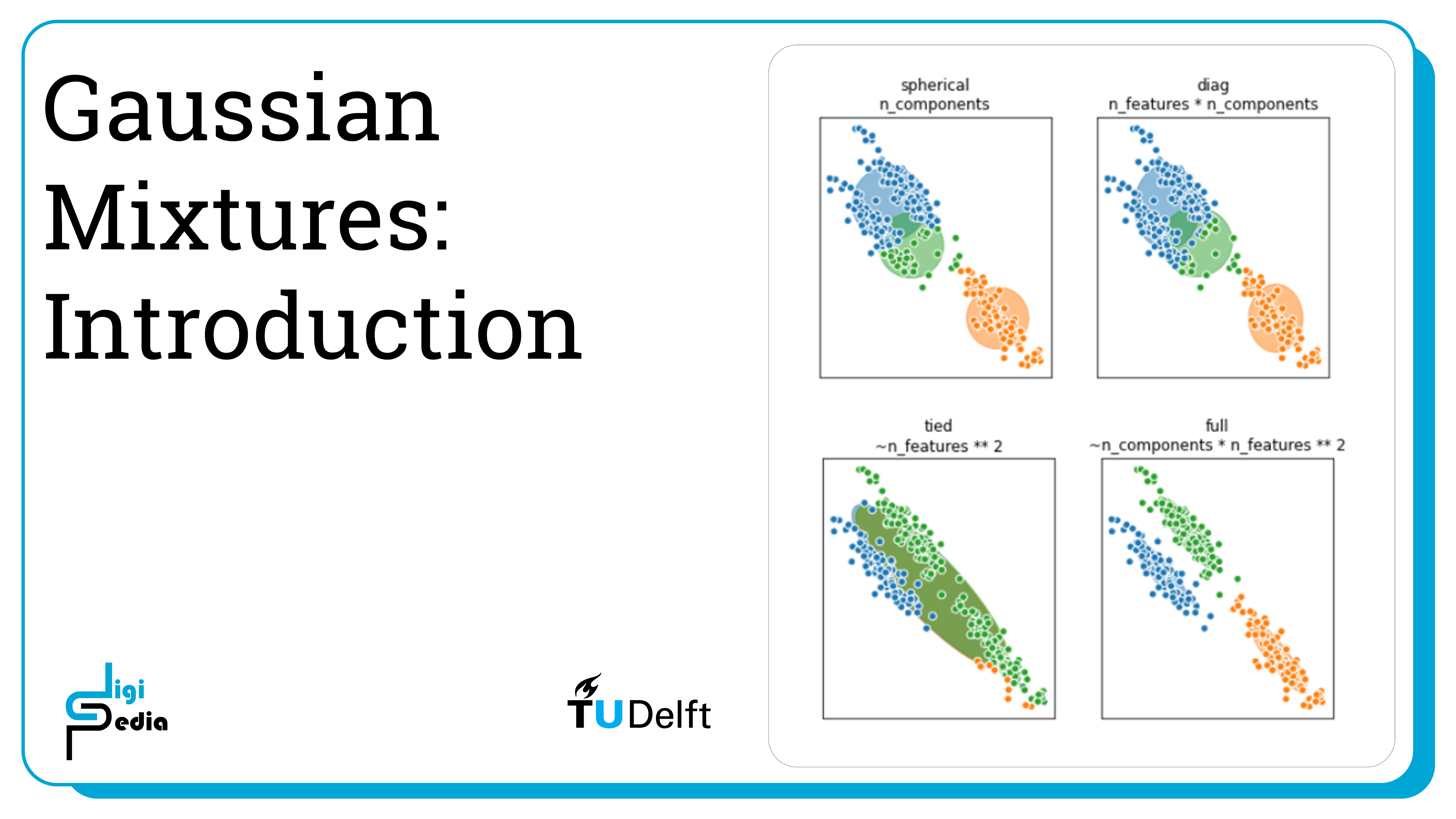
Gaussian Mixture is a type model corresponding to the probability distribution of a collection of data points within the data set. It is a probabilistic model which assumes that the data points are generated from a mixture of a finite number of Gaussian distributions with unknown parameters.
Gaussian Mixture uses an EM (Expectation-Maximization) algorithm to determine the parameters. The algorithm starts from an initial estimate of the density contours which can be controlled by the init_params parameter in SciKit Learn. The options are kmeans, k-means ++, random, and random_from_data. The algorithm then proceeds to update the density contours until convergence. Each iteration consists of an E-step and an M-step.
- E-step: compute the membership weights for all data points and density contours (weights of Gaussians)
- M-step: use the membership weights to calculate new density contours (parameters of Gaussians)
EM steps are continuously taken until a stopping condition has been reached. It is possible to think of mixture models as a method to incorporate information about the covariance structure of the data and the centers of the latent Gaussians into k-means, thereby extending upon K-Means clustering.
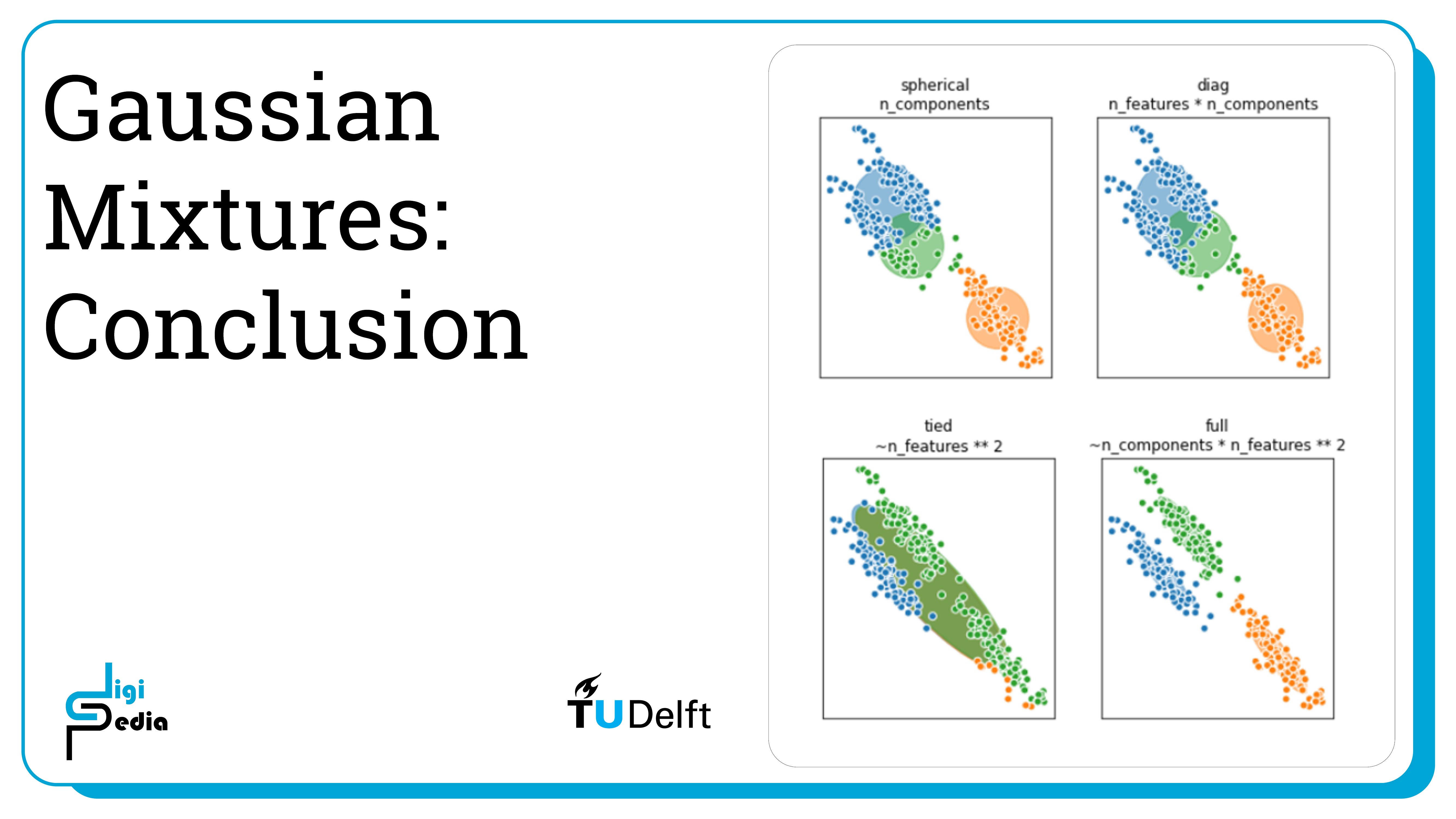
Covariance is determined by the covariance_type parameter in SciKit Learn. In Gaussian Mixtures, the density contours are ellipsoids. The covariance determines the directions and the lengths of the axes of these density contours. SciKit Learn allows for use of four different types of covariance including diagonal, spherical, tied and full covariance. These are demonstrated in the next chapters.
Gaussian Mixtures 2/3
Notebooklink copied
Dataset
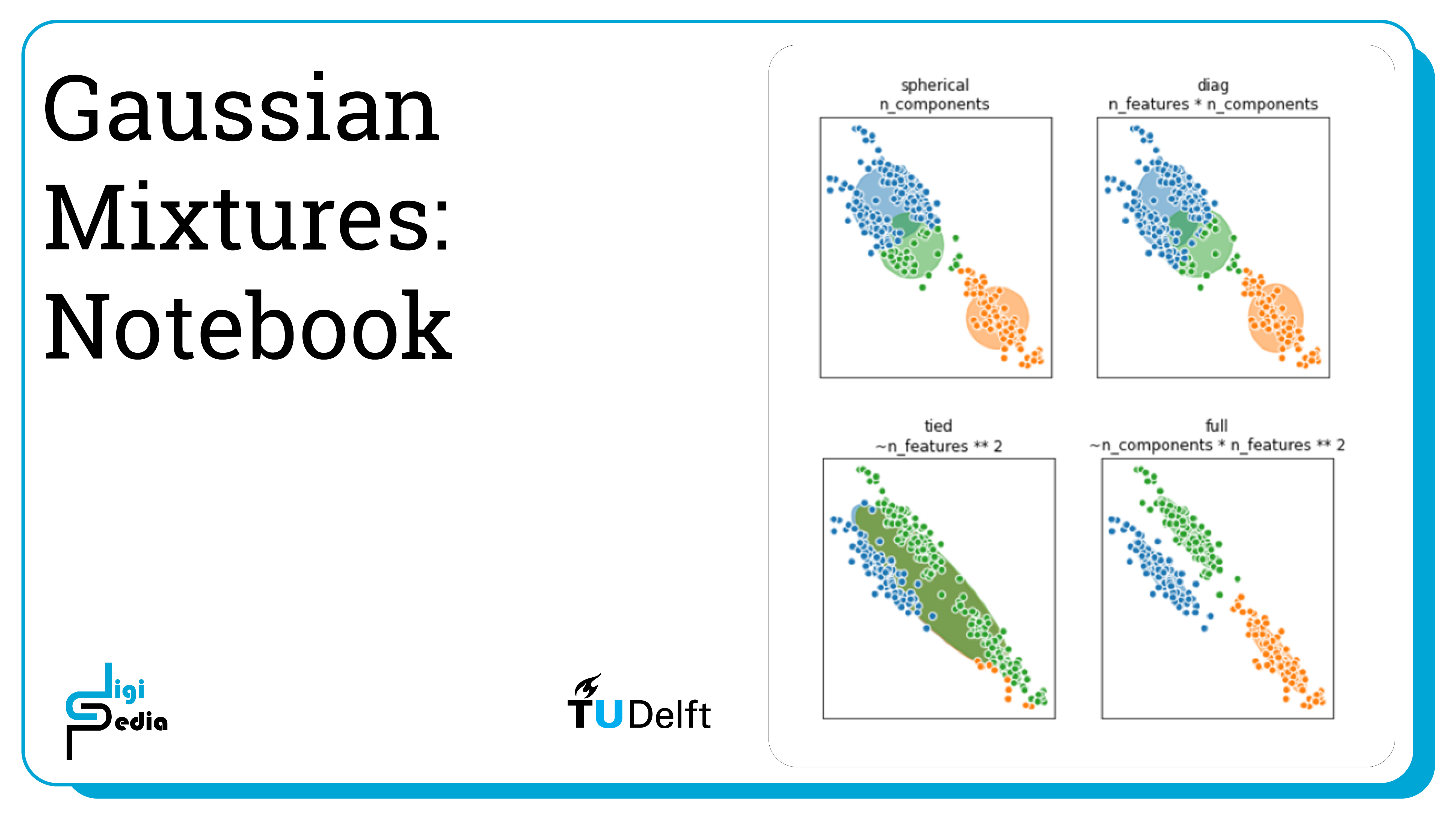
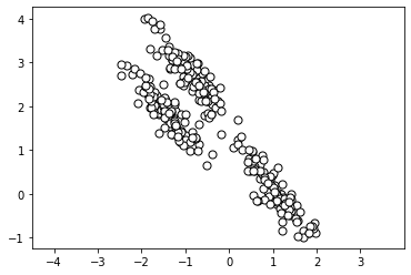
For this notebook, we will use a generated dataset in the shape of elongated clusters. We can generate and visualize the dataset below.
import numpy as np
import matplotlib.pyplot as plt
from sklearn.datasets import make_blobs

# create dataset and stretch to create non-spherical clusters
X, y = make_blobs(
n_samples=300, centers=3,
cluster_std=0.60, random_state=0
)
rng = np.random.RandomState(13)
X_stretched = np.dot(X, rng.randn(2, 2))

plt.scatter(
X_stretched[:, 0], X_stretched[:, 1],
c='white', marker='o',
edgecolor='black', s=50
)
plt.axis('equal')
plt.show()
K-Means
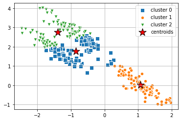
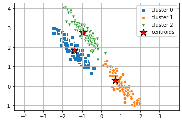
As discussed in the previous notebook, K-Means works best for spherical clusters. When the dataset is stretched like it is above, K-Means does not identify the clusters. This is where other clustering methods, like Gaussian Mixture help. Below, we can see that K-Means does not properly cluster the data.
from sklearn.cluster import KMeans

clusters = 3
km = KMeans( n_clusters=clusters,
     init='random',
     n_init=10,
     max_iter=300,
     tol=1e-04, random_state=0 )

y_km = km.fit_predict(X_stretched)
# plot the 3 clusters
markers = ['s', 'H', 'v', 'p', '^', 'o', 'X', 'd', 'P' ]
for i in range(clusters):
plt.scatter(
X_stretched[y_km == i, 0], X_stretched[y_km == i, 1],
s=50,
marker=markers[i], edgecolor='white',
label='cluster ' + str(i)
)
# plot the centroids
plt.scatter(
km.cluster_centers_[:, 0], km.cluster_centers_[:, 1],
s=250, marker='*',
c='red', edgecolor='black',
label='centroids'
)
plt.legend(scatterpoints=1)
plt.grid()
plt.show()
Gaussian Mixture
When we apply Gaussian Mixture with the full covariance type to the same dataset, we can see that the clusters created align with the clusters we can visually separate.
from sklearn.mixture import GaussianMixture

clusters_gm = 3
gmm = GaussianMixture(n_components=clusters_gm, covariance_type='full', random_state=2, init_params='random')
import scipy.stats
y_gmm = gmm.fit(X_stretched).predict(X_stretched)
# plot the clusters
markers = ['s', 'H', 'v', 'p', '^', 'o', 'X', 'd', 'P' ]
centers = np.empty(shape=(gmm.n_components, X.shape[1]))
for i in range(gmm.n_components):
density = scipy.stats.multivariate_normal(cov=gmm.covariances_[i], mean=gmm.means_[i]).logpdf(X)
centers[i, :] = X[np.argmax(density)]
for i in range(clusters_gm):
plt.scatter(
X_stretched[y_gmm == i, 0], X_stretched[y_gmm == i, 1],
s=50,
marker=markers[i], edgecolor='white',
label='cluster ' + str(i)
)
# plot the centroids
plt.scatter(
centers[:, 0], centers[:, 1],
s=250, marker='*',
c='red', edgecolor='black',
label='centroids'
)
plt.legend(scatterpoints=1)
plt.axis('equal')
plt.grid()
plt.show()
Covariance
As discussed earlier, the covariance adjusts the directions and lengths of the axes of the ellipsoidal density contours. SciKit Learn has four different parameter values for the covariance. They are diagonal, spherical, tied and full covariance and are visualized below.
import matplotlib as mpl
import matplotlib.pyplot as plt
import numpy as np
from sklearn.mixture import GaussianMixture

#Code adjusted from example by Andreas Mueller https://github.com/scikit-learn/scikit-learn/issues/10863

def make_ellipses(gmm, ax):
    for n in range(gmm.n_components):
        if gmm.covariance_type == 'full':
            covariances = gmm.covariances_[n]
        elif gmm.covariance_type == 'tied':
            covariances = gmm.covariances_
        elif gmm.covariance_type == 'diag':
            covariances = np.diag(gmm.covariances_[n])
        elif gmm.covariance_type == 'spherical':
            covariances = np.eye(gmm.means_.shape[1]) * gmm.covariances_[n]
        v, w = np.linalg.eigh(covariances)
        u = w[0] / np.linalg.norm(w[0])
        angle = np.arctan2(u[1], u[0])
        angle = 180 * angle / np.pi  # convert to degrees
        v = 2. * np.sqrt(2.) * np.sqrt(v)
        ell = mpl.patches.Ellipse(gmm.means_[n], v[0], v[1],
                                  180 + angle, color=plt.cm.tab10(n))
        ell.set_clip_box(ax.bbox)
        ell.set_alpha(0.5)
        ax.add_artist(ell)

# Try GMMs using different types of covariances.
estimators = [GaussianMixture(n_components=3, covariance_type=cov_type, random_state=2, init_params='random')
              for cov_type in ['spherical', 'diag', 'tied', 'full']]

n_estimators = len(estimators)

fig, axes = plt.subplots(1, 4, figsize=(15, 5))
titles = ("spherical\nn_components", "diag\nn_features * n_components",
          "tied\n~n_features ** 2", "full\n~n_components * n_features ** 2")

for ax, title, estimator in zip(axes, titles, estimators):
    estimator.fit(X_stretched)

    make_ellipses(estimator, ax)

    pred = estimator.predict(X_stretched)
    ax.scatter(X_stretched[:, 0], X_stretched[:, 1], c=plt.cm.tab10(pred), edgecolor='white')

    ax.set_xticks(())
    ax.set_yticks(())
    ax.set_title(title)
    ax.set_aspect("equal")
TASK: Choose two features from the wine dataset which are appropriate for clustering using gaussian mixture and apply it on the data based on those two features.
Don’t forget to normalize the input data using a pipeline like we have done in previous notebooks. Check the SVM notebook for an example.
Gaussian Mixtures 3/3
Conclusionlink copied
- Gaussian Mixtures assume the dataset is described by a finite numbers of weighted Gaussians
- Expectation-Maximization is used to determined the weights and mean/covariances of the Gaussians
- The initial centroids, controlled by the init_params parameter in SciKit Learn allow for initialization using kmeans, kmeans++, random, and random_from_data
- Each iteration consists of an E-step and an M-step:
- E-step: compute the membership weights for all data points and centroids
- M-step: use the membership weights to calculate a new centroid
- Mixture models generalize K-Means clustering by incorporating information about the covariance structure of the data and the centers of the latent Gaussians
- The covariance adjusts the directions and lengths of the axes of the ellipsoidal density contours
- SciKit Learn has four different parameter values for the covariance: diagonal, spherical, tied and full covariance
Write your feedback.
Write your feedback on "Gaussian Mixtures"".
If you're providing a specific feedback to a part of the chapter, mention which part (text, image, or video) that you have specific feedback for."Thank your for your feedback.
Your feedback has been submitted successfully and is now awaiting review. We appreciate your input and will ensure it aligns with our guidelines before it’s published.
