Naive Bayes Classifiers (Multi-label)
-
Intro
-
Introduction & Dataset
-
Train Test
-
Conclusion
Information
| Primary software used | Jupyter Notebook |
| Course | Naive Bayes Classifiers (Multi-label) |
| Primary subject | AI & ML |
| Secondary subject | Machine Learning |
| Level | Beginner |
| Last updated | November 19, 2024 |
| Keywords |
Responsible
| Teachers | |
| Faculty |
Naive Bayes Classifiers (Multi-label) 0/3
Naive Bayes Classifiers (Multi-label)
In this tutorial the theory of Naive Bayes Classifiers is explained with an example of multilabel.
Bayes Theorem The probability of an event taking place considering prior knowledge about features that might impact the event. describes the probability of an event taking place considering prior knowledge about features that might impact the event. Naive Bayes classifiers are based on Bayes theorem and assumes each feature is independent given that the class is known. In other words, the classifier assumes that one feature being present in a class is not related to another feature being present in the same class. Features can be discrete or continuous. This tutorial reviews classification of multiple labels.
For this tutorial you need to have installed Python, Jupyter notebooks, and some common libraries including Scikit Learn. Please see the following tutorial for more information.
Steps followed to create a Naive Bayes classifier (binary) in this notebook:
- Get encoded dataset
- Split dataset into training and test data
- Create model
- Evaluate model
Exercise file
You can download the notebook version here:
Naive Bayes Classifiers (Multi-label) 1/3
Introduction & Datasetlink copied
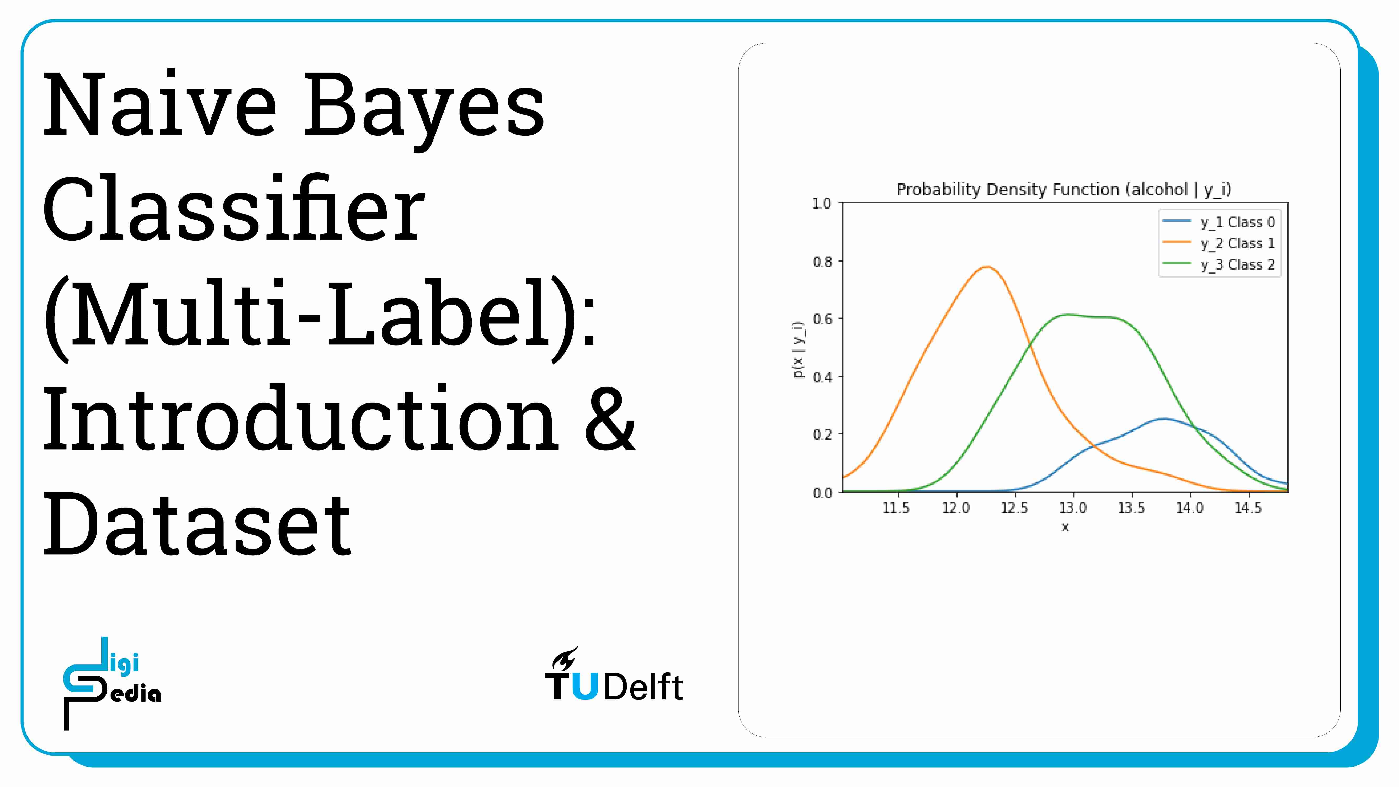
Naive Bayes classifiers for multiple labels work similar to naive Bayes classifiers for two classes. In this case, we will be looking 13 different features of wine: alcohol, malic acid, ash, alcalinity of ash, magnesium, total phenols, flavanoids, nonflavanoid phenols, proanthocyanins, color intensity, hue, od280/od315 of diluted wines, and proline. Based on these 13 features, the wine will be categorized into three classes: Class 0 (y1), Class 1 (y2), and Class 2 (y3). This time, the features are continuous, not discrete.
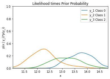
Again, the priors, or the probabilities of wine being assigned to a particular class, must be known. For the example below, the data is available for 178 wines. 59 wines were classified as Class 0 (y1) so the probability of the wine being assigned to Class 0 (P(y1)), is equal to 59/178. 71 wines were classified as Class 1 (y2) so the probability of the wine being assigned to Class 1 (P(y2)), is equal to 71/178. 48 wines were classified as Class 2 (y3) so the probability of the wine being assigned to Class 2 (P(y3)), is equal to 48/178.
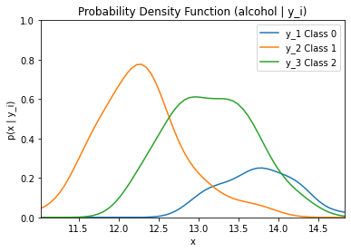
Because the dataset uses continuous features, the likelihood is represented by the probability density function (p(X|yi) where i = 1, 2, 3).The process is similar to classifying into two classes except now look at the probability of three classes.
- If P(y2|X) < P(y1|X) and P(y3|X) < P(y1|X), assign sample X to y1
If the probability of the wine being of Class 0 given the features is greater than the probability of the wine being of Class 1 and is greater than the probability of the wine being of Class 2, then the features are assigned to Class 0.
- If P(y1|X) < P(y2|X) and P(y3|X) < P(y2|X), assign sample X to y2
If the probability of the wine being of Class 1 given the features is greater than the probability of the wine being of Class 0 and is greater than the probability of the wine being of Class 2, then the features are assigned to Class 1.
- If P(y1|X) < P(y3|X) and P(y2|X) < P(y3|X), assign sample X to y3
If the probability of the wine being of Class 2 given the features is greater than the probability of the wine being of Class 0 and is greater than the probability of the wine being of Class 1, then the features are assigned to Class 2.
Let’s take a look at implementing a naive Bayes Classifier with more than two classes with SciKit Learn.
Load the wine dataset and assign it to a variable. Print the name of the featues and labels to see the features and classes of the dataset.
To see the output of the following cells, please see the Jupyter notebook.
# Import scikit-learn dataset library
from sklearn import datasets
from scipy.stats.kde import gaussian_kde
import numpy as np
import matplotlib.pyplot as plt

# Load dataset
wine = datasets.load_wine()

# print the names of the 13 features
print("Features: ", wine.feature_names)

# print the label type of wine(class_0, class_1, class_2)
print("Labels: ", wine.target_names)
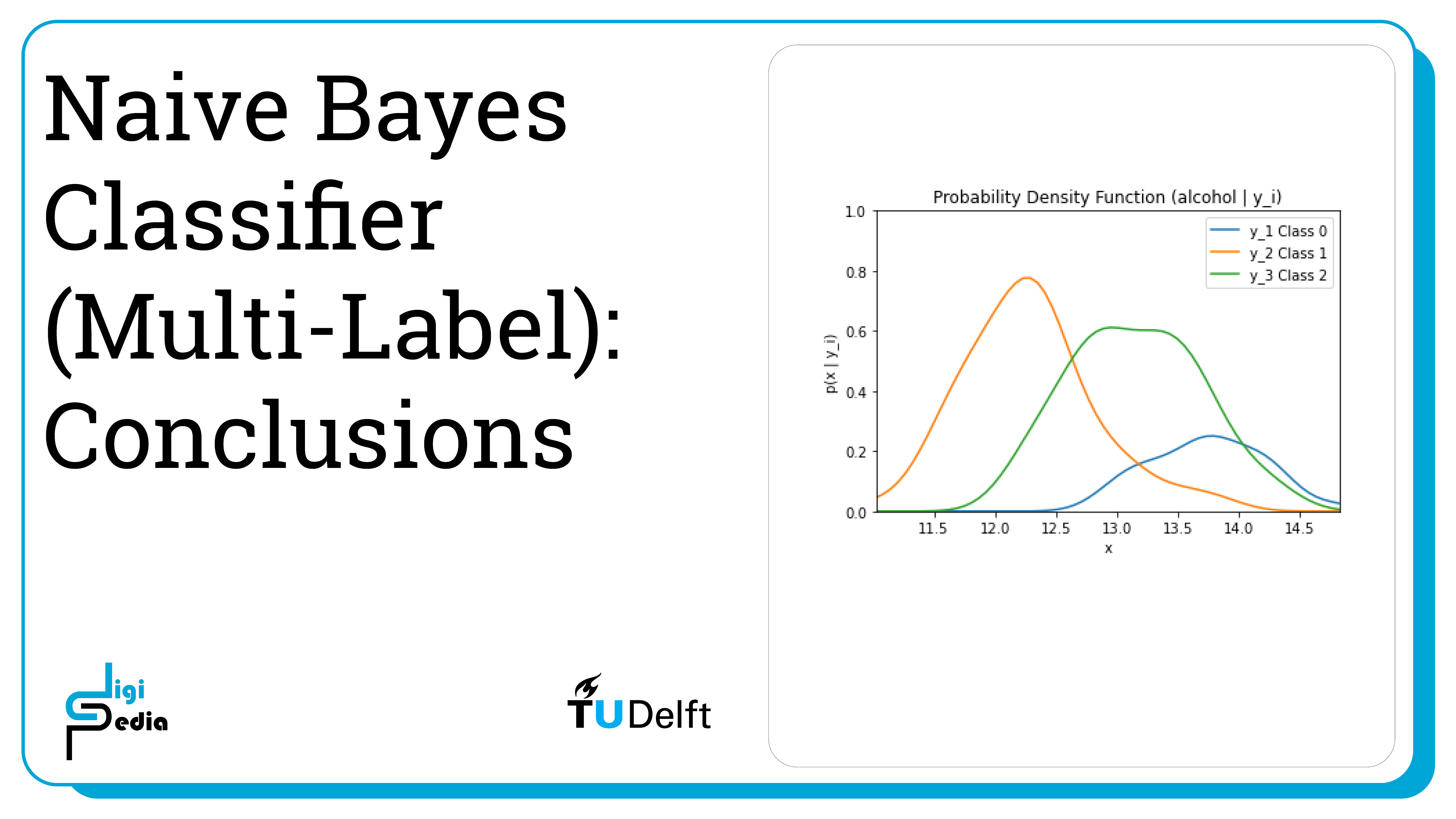
By running the code below, the likelihood of the feature alcohol given the three classes (0, 1, and 2) is graphed. The likelihood is represented by the probability mass function (p(X|y1)).
alcohol = wine.data[:, 0]
classes = wine.target

alcohol_class0 = [w[0] for w in zip(alcohol, classes) if w[1] == 0]
alcohol_class1 = [w[0] for w in zip(alcohol, classes) if w[1] == 1]
alcohol_class2 = [w[0] for w in zip(alcohol, classes) if w[1] == 2]
classes_all = ["Class 0", "Class 1", "Class 2"]

kde_0 = gaussian_kde(alcohol_class0)
dist_space_0 = np.linspace(0, 15, 250)
kde_1 = gaussian_kde(alcohol_class1)
dist_space_1 = np.linspace(0, 15, 250)
kde_2 = gaussian_kde(alcohol_class2)
dist_space_2 = np.linspace(0, 15, 250)

# plot the results
plt.title('Probability Density Function (alcohol | y_i)')
plt.ylim((0, 1))plt.xlim((np.amin(alcohol), np.amax(alcohol)))
plt.xlabel('x') plt.ylabel('p(x | y_i)')
plt.plot(dist_space_0, kde_0(dist_space_0), label='y_1 Class 0')
plt.plot(dist_space_1, kde_1(dist_space_1), label='y_2 Class 1')
plt.plot(dist_space_2, kde_2(dist_space_2), label='y_3 Class 2')
plt.legend()
plt.show()
By running the code below, the likelihood of the feature alcohol given the three classes (0, 1, and 2) multiplied by the priors of each class is graphed.
alcohol = wine.data[:, 0]
classes = wine.target

alcohol_class0 = [w[0] for w in zip(alcohol, classes) if w[1] == 0]
alcohol_class1 = [w[0] for w in zip(alcohol, classes) if w[1] == 1]
alcohol_class2 = [w[0] for w in zip(alcohol, classes) if w[1] == 2]
classes_all = ["Class 0", "Class 1", "Class 2"]

kde_0 = gaussian_kde(alcohol_class0)
dist_space_0 = np.linspace(0, 15, 250)
kde_1 = gaussian_kde(alcohol_class1)
dist_space_1 = np.linspace(0, 15, 250)
kde_2 = gaussian_kde(alcohol_class2)
dist_space_2 = np.linspace(0, 15, 250)

# plot the results
plt.title('Likelihood * Class Priors')
plt.ylim((0, 1))
plt.xlim((np.amin(alcohol), np.amax(alcohol)))
plt.xlabel('x')
plt.ylabel('p(x | y_i)*p(y_i)')
plt.plot(dist_space_0, kde_0(dist_space_0) * (len(alcohol_class0) / len(alcohol)), label='y_1 Class 0')
plt.plot(dist_space_1, kde_1(dist_space_1) * (len(alcohol_class1) / len(alcohol)), label='y_2 Class 1')
plt.plot(dist_space_2, kde_2(dist_space_2) * (len(alcohol_class2) / len(alcohol)), label='y_3 Class 2')
plt.legend()
plt.show()
We can print a number of pieces of information to understand some of the characteristics of the dataset.
For the output of the following cells, please see the jupyter notebook.
print("Class 0 count: ", np.count_nonzero(wine.target == 0))
print("Class 1 count: ", np.count_nonzero(wine.target == 1))
print("Class 2 count: ", np.count_nonzero(wine.target == 2))
print("Total wines for classification: ", len(wine.target))

Class 0 count: 59
Class 1 count: 71
Class 2 count: 48
Total wines for classification: 178

# print data(feature)shape
wine.data.shape
# print the wine data features (top 5 records)
print(wine.data[0:5])# try printing the top 5 records using pandas for a easier to read display
import pandas as pd
df = pd.DataFrame(wine.data[0:5], columns = wine.feature_names)
df.head()# print the wine labels (0:Class_0, 1:class_2, 2:class_2)
print(wine.target)Naive Bayes Classifiers (Multi-label) 2/3
Train Testlink copied
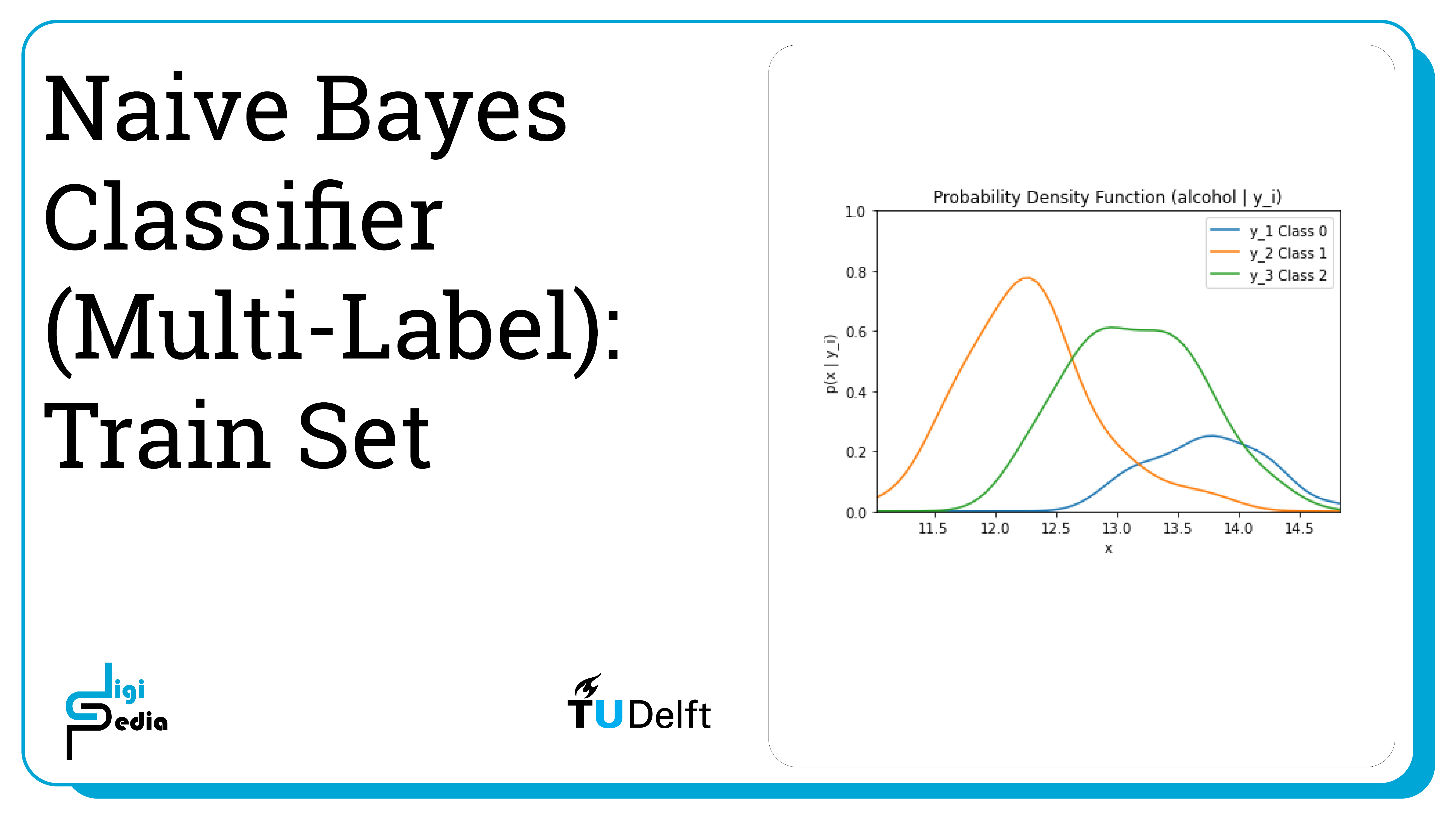
The accuracy of a classification model is the number of correct predictions divided by the total number of predictions. This statistic is used to describes the model’s performance. To determine accuracy, it is necessary to split the dataset into train and test data. Training and testing on the same dataset will result in a well-trained classifier but the accuracy of the model will be biased. A test set that is too small may result in an unbiased but unreliable accuracy estimate for a well-trained classifier. A test set that is too large may result in an unbiased and reliable accuracy for a badly trained classifier. This is why the consideration of train and test sets is important to consider. Common train to test ratios include 8:2, 7:3, and 6:4.Below, split the data into training and test sets with a 7:3 ratio, train the model on the training dataset, and then check the accuracy on the test dataset.
# Import train_test_split function
from sklearn.model_selection import train_test_split

# Split dataset into training set and test set
X_train, X_test, y_train, y_test = train_test_split(wine.data, wine.target, test_size=0.3,random_state=109) # 70% training and 30% test

# Import Gaussian Naive Bayes model
from sklearn.naive_bayes import GaussianNB

# Create a Gaussian Classifier
gnb = GaussianNB()

# Train the model using the training sets
gnb.fit(X_train, y_train)

# Predict the response for test dataset
y_pred = gnb.predict(X_test)
Predict a single output with the model.
new_datapoint = wine.data[13, :]


# Predict Output
predicted= gnb.predict([new_datapoint])
predict_probability = gnb.predict_proba([new_datapoint])
print("Predicted Value:", predicted, " with ", predict_probability)
The output is:
Predicted Value: [0] with [[1.00000000e+00 3.95539110e-12 6.25476571e-44]]
Print the accuracy of a classification model using the accuracy_score method.
# Import scikit-learn metrics module for accuracy calculation
from sklearn import metrics

# Model Accuracy, how often is the classifier correct?
print("Accuracy:",metrics.accuracy_score(y_test, y_pred))
The output is:
Accuracy: 0.9074074074074074
Print the confusion matrix to see which classes are commonly misclassified. The columns represent the actual values and the rows represent the classified values. So the diagonal numbers show the number of correctly classified data.A
# Import scikit-learn metrics module for confusion matrix
from sklearn import metrics

# Which classes are commonly misclassified?
print(metrics.confusion_matrix(y_test, y_pred, labels=[0, 1, 2]))
The output is:
[[20 1 0]
[ 2 15 2]
[ 0 0 14]]
Naive Bayes Classifiers (Multi-label) 3/3
Conclusionlink copied
- Continuous features can be measured on a scale and can be divided into smaller parts
- The likelihood is expressed by the probability density function for continuous features
- Print characteristics like the probability density function, the priors, and some of the datapoints to better understand the dataset
- The accuracy of a classification model is the number of correct predictions divided by the total number of predictions. This statistic is used to describe the model’s performance.
- To determine accuracy, it is necessary to split the dataset into train and test data. The ratio has an impact on how well-trained the model is an how biased the accuracy prediction is. Common train to test ratios include 8:2, 7:3, and 6:4
- After the classifier is trained on the training data, it can predict the classification of the test data. The accuracy_score method returns the accuracy of the trained model
Write your feedback.
Write your feedback on "Naive Bayes Classifiers (Multi-label)"".
If you're providing a specific feedback to a part of the chapter, mention which part (text, image, or video) that you have specific feedback for."Thank your for your feedback.
Your feedback has been submitted successfully and is now awaiting review. We appreciate your input and will ensure it aligns with our guidelines before it’s published.
