Multinomial Logistic Regression
-
Intro
-
Notebook
-
Conclusion
Information
| Primary software used | Jupyter Notebook |
| Course | Multinomial Logistic Regression |
| Primary subject | AI & ML |
| Secondary subject | Machine Learning |
| Level | Beginner |
| Last updated | November 11, 2024 |
| Keywords |
Responsible
| Teachers | |
| Faculty |
Multinomial Logistic Regression 0/2
Multinomial Logistic Regression
Machine Learning method to classify linearly separable classes.
Multinomial logistic regression is a type of regression analysis used for predicting the probabilities of different possible outcomes of a categorical dependent variable with more than two classes. It extends binary logistic regression by using a softmax function to model the relationship between multiple classes and predictor variables, allowing for the prediction of probabilities for each class.
For this tutorial you need to have installed Python, Jupyter notebooks, and some common libraries including Scikit Learn. Please see the following tutorial for more information.

Multinomial Logistic Regression is used to classify linearly separable classes. It predicts the probability of the class of a categorical variable given a set of variables (features). Multinomial Logistic Regression extends the application of Logistic Regression to more than two classes.
Logistic Regression is a binary classifier so it classifies data into two classes. The classifier outputs the probability mass function of a datapoint over the classes, namely, a vector of values stating the probability of the datapoint belonging to each class. If the probability is above a specific threshold, it will assign the datapoint to that class. Multinomial Logistic Regression uses the same process but for more than two classes. In this notebook, we see how to implement multinomial logistic regression using the wine dataset from SciKit Learn.
Exercise file
You can download the notebook file here:
Multinomial Logistic Regression 1/2
Notebooklink copied
Loading the dataset
Load the dataset and print some the information about the dataset. Please see the notebook for the output of these cells.
# Import scikit-learn dataset library
from sklearn import datasets

# Load dataset
wine = datasets.load_wine()

# print the names of the features
print(wine.feature_names)
Feature Insight
We can get insight on the data in the dataset by printing the dataset properties and variables.
# print the label species (class_0, class_1, class_2)
print(wine.target_names)
# print the wine data (top 5 records)
print(wine.data[0:5])# print the wine labels (0:Class_0, 1:Class_1, 2:Class_3)
print(wine.target)# print data(feature)shape
print(wine.data.shape)
# print target(or label)shape
print(wine.target.shape)
Train model with one feature
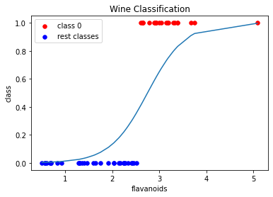
First, we will train the classifier and predict the classes of the data using only one feature so we can visualize the probability curve for the data.
# import the class
from sklearn.model_selection import train_test_split
from sklearn.linear_model import LogisticRegression
from sklearn import preprocessing
from sklearn import metrics

#feature 6, flavanoids, results in highest accuracy (78%), feature 0, alcohol, also has fairly high accuracy (74%)
feature = 6

# Split dataset into training set and test set
X_train, X_test, y_train, y_test = train_test_split(wine.data[:, feature].reshape(-1, 1), wine.target, test_size=0.3) # 70% training and 30% test

# instantiate the model (using the default parameters)
logreg = LogisticRegression(multi_class="multinomial", max_iter=10000)

# fit the model with data
logreg.fit(X_train, y_train)

y_pred = logreg.predict(X_test)

print("Accuracy:",metrics.accuracy_score(y_test, y_pred))

cnf_matrix = metrics.confusion_matrix(y_test, y_pred)
print("Confusion Matrix:", cnf_matrix)
The output:
Accuracy: 0.6851851851851852
Confusion Matrix:
[[13 4 0]
[ 9 15 4]
[ 0 0 9]]
import numpy as np
import matplotlib.pyplot as plt
import math

# plot class 0 versus the rest to show probability curve
# update list so 0 is class 0 and 1 is "rest"
y_pred_class0 = [1 for x in y_pred if x == 0]
y_pred_classrest = [0 for x in y_pred if x > 0]

X_class0 = [X_test[i, 0] for i, x in enumerate(y_pred) if x == 0]
X_classrest = [X_test[i,0] for i, x in enumerate(y_pred) if x != 0]

X_value = X_test[:,0]
X_value.sort()
sigmoid = [1/(1+math.exp(2.5*-(x-2.75))) for x in X_value]

plt.scatter(X_class0, y_pred_class0, s=30, c='r', label='class 0')
plt.scatter(X_classrest, y_pred_classrest, s=30, c='b', label='rest classes')
plt.plot(X_value,sigmoid)

plt.title('Wine Classification')
plt.xlabel('flavanoids')
plt.ylabel('class')
plt.legend()
plt.show()

Train Model with all Features
Now, train a classifier and predict the classes of the data. Split the data into a train and test set based on a 70/30 split.
# Import train_test_split function
from sklearn.model_selection import train_test_split

# Split dataset into training set and test set
X_train, X_test, y_train, y_test = train_test_split(wine.data, wine.target, test_size=0.3) # 70% training and 30% test

# import the class
from sklearn.linear_model import LogisticRegression
from sklearn import preprocessing

# instantiate the model (using the default parameters)
logreg = LogisticRegression(multi_class="multinomial", max_iter=10000)

# fit the model with data
logreg.fit(X_train, y_train)

y_pred = logreg.predict(X_test)
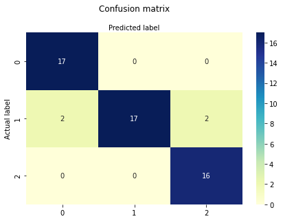
Check the performance of the model by printing the confusion matrix and also plotting the confusion matrix.
# import the metrics class
from sklearn import metrics

print("Accuracy:",metrics.accuracy_score(y_test, y_pred))

cnf_matrix = metrics.confusion_matrix(y_test, y_pred)
print("Confusion Matrix:", cnf_matrix)
The output:
Accuracy: 0.9259259259259259
Confusion Matrix:
[[17 0 0]
[ 2 17 2]
[ 0 0 16]]
# import required modules
import numpy as np
import matplotlib.pyplot as plt
import seaborn as sns
import pandas as pd

class_names=[0,1,2] # name of classes
fig, ax = plt.subplots()
tick_marks = np.arange(len(class_names))
plt.xticks(tick_marks, class_names)
plt.yticks(tick_marks, class_names)

# create heatmap
sns.heatmap(pd.DataFrame(cnf_matrix), annot=True, cmap="YlGnBu" ,fmt='g')
ax.xaxis.set_label_position("top")
plt.tight_layout()
plt.title('Confusion matrix', y=1.1)
plt.ylabel('Actual label')
plt.xlabel('Predicted label')
Evaluate model performance
To evaluate the performance of multinomial logistic regression, it is possible to use similar metrics to those used before, like checking the accuracy and printing a confusion matrix. Through SciKit Learn, it is also possible to get the precision, recall, and f1-score of each class. Precision
- Precision: is the number of true positive results divided by the total predicted positive values
- The total predicted positive values is the sum of the number of true positive results and the false positive results
- For multiple classes, it is the number of correctly classified samples of that class divided by the total number of samples that the classifier assigned to that class
Recall
- Recall: is the number of true positive results divided by the total number of positive results
- The total positive results is the sum of the number of true positive results and the false negative results
- For multiple classes, it is the number of correctly classified samples of that class divided by the total number of samples that actually belong to that class
F-score
- F-score is equal to two times the precision times the recall divided by the precision plus the recall
F-score = 2 * (precision * recall) / (precision + recall)
from sklearn.metrics import classification_report
print(classification_report(y_test, y_pred, target_names=wine.target_names))
The output:
precision recall f1-score support
class_0 0.89 1.00 0.94 17
class_1 1.00 0.81 0.89 21
class_2 0.89 1.00 0.94 16
accuracy 0.93 54
macro avg 0.93 0.94 0.93 54
weighted avg 0.93 0.93 0.92 54Multinomial Logistic Regression 2/2
Conclusionlink copied
- Classifies linearly separable classes (can use non-linear transformations for non-linearly seperable classes)
- Predicts the probability of the class of a categorically distributed variable (datapoint) given a set of variables (features)
- Logistic Regression is used for classifying data with two classes, multinomial logistic regression is used for classifying data with more than two classes
Write your feedback.
Write your feedback on "Multinomial Logistic Regression"".
If you're providing a specific feedback to a part of the chapter, mention which part (text, image, or video) that you have specific feedback for."Thank your for your feedback.
Your feedback has been submitted successfully and is now awaiting review. We appreciate your input and will ensure it aligns with our guidelines before it’s published.
