Multi-Objective Optimisation – Indoor Daylight
-
Intro
-
Design
-
Tutorial Steps
-
Simulation Set-Up
-
Optimization Set-Up and Run
-
Conclusion
-
Useful Links
Information
| Primary software used | Grasshopper |
| Course | Multi-Objective Optimisation – Indoor Daylight |
| Primary subject | Analysis & simulation |
| Secondary subject | Optimization |
| Level | Intermediate |
| Last updated | December 6, 2024 |
| Keywords |
Responsible
| Teachers | |
| Faculty |
Multi-Objective Optimisation – Indoor Daylight 0/6
Multi-Objective Optimisation – Indoor Daylight
In this tutorial you will learn how to make use of the powerful Wallacei plugin multi objective optimisation capabilities in the case of indoor daylight simulation.
In this tutorial you will learn how to make use of the powerful Wallacei plugin multi objective optimisation capabilities in the case of indoor daylight simulation. You will learn how to combine environmental simulation engine (Ladybug + Honeybee) with the genetic algorithm functionality embedded in Wallacei to find the most optimal outcomes.
This tutorial is from Wallacei series of tutorials and is based on the “HB Daylight Simulation” and “Honeybee model set-up” tutorials.
Multi-Objective Optimisation – Indoor Daylight 1/6
Designlink copied
The example used in this tutorial is a slightly modified version of the shoebox room from the “HB Daylight Simulation” tutorial. It is a shoebox geometry of an apartment which is on the ground floor of a 2-storeys building. It has a rectangular plan of 10m*10m and it has a height of 3m.
The apartment has two windows on one of the walls, each of them is equipped with horizontal wooden louvers as shadings. On the left and right side there are adjacent apartments, but on the back side it is not neighboring any other apartment or building.
The exterior walls are made of concrete in light grey colour. The slabs are also made of concrete and they are painted in white colour on the bottom side (ceiling). On the top part (floor), they are covered by timber in a darker colour. The interior walls are made of plywood and covered also in white paint.
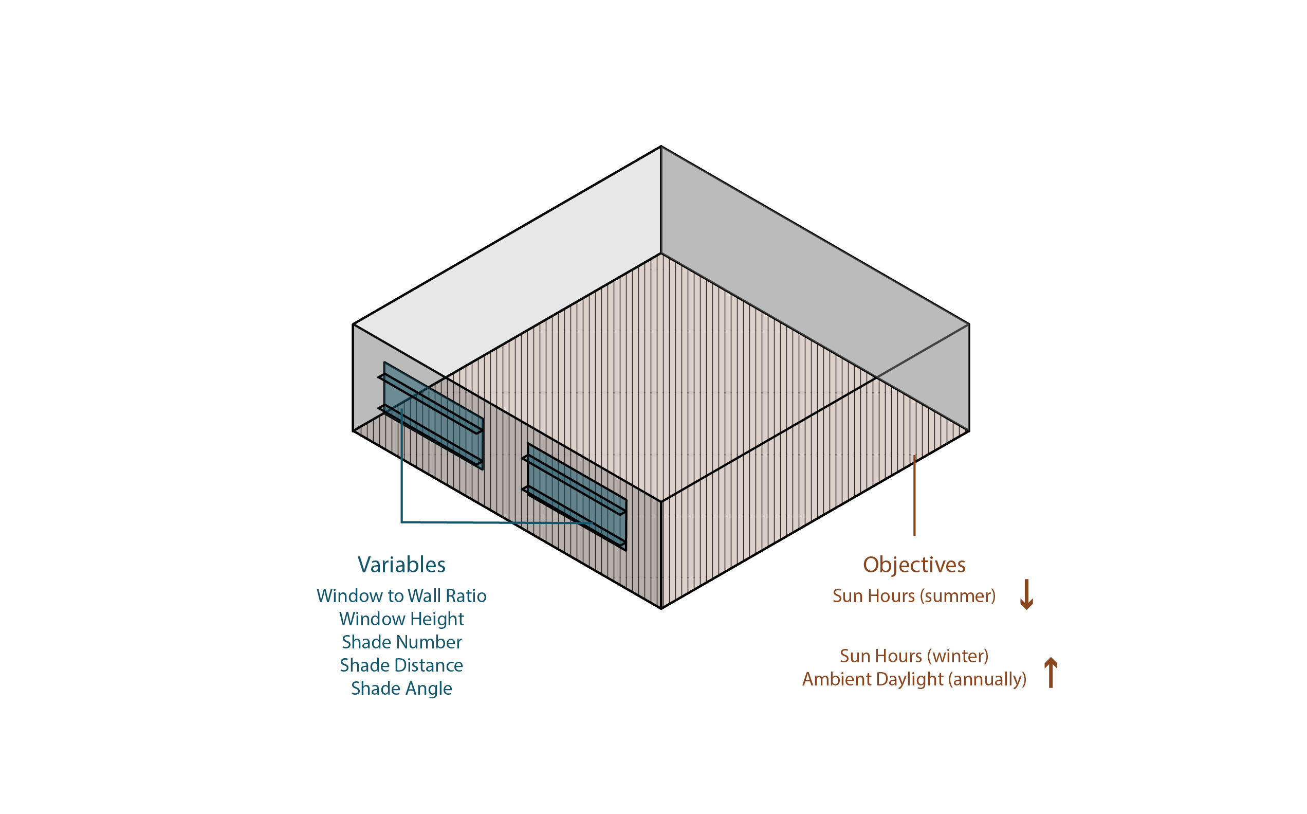
We are going to optimize interior daylight conditions; our objectives will be:
- minimize total sun hours in the summer period,
- maximize total sun hours in winter,
- maximize annual Ambient Daylight.
Our variables will be:
- window to wall ratio
- window height
- number of shadings
- distance between shadings
- shadings angle
Exercise file
As a starting point for this tutorial, you’ll need a slightly trimmed down and modified version of the “HB Daylight Simulation” grasshopper script. We will add necessary components in the following steps.
Multi-Objective Optimisation – Indoor Daylight 2/6
Tutorial Stepslink copied
Geometry Setup for HB Room
Let’s start with setting up the honeybee geometry. We need a box shaped room with two exterior walls and two interior ones. On one of the exterior walls, we need two windows, which are equipped with horizontal louver shadings. We want to control parameters like window to wall ratio, louver count, etc. – listed before.
We are going to start with already existing part of the grasshopper script from the “HB Daylight Simulation”. You can download the starting file here: gh_file.
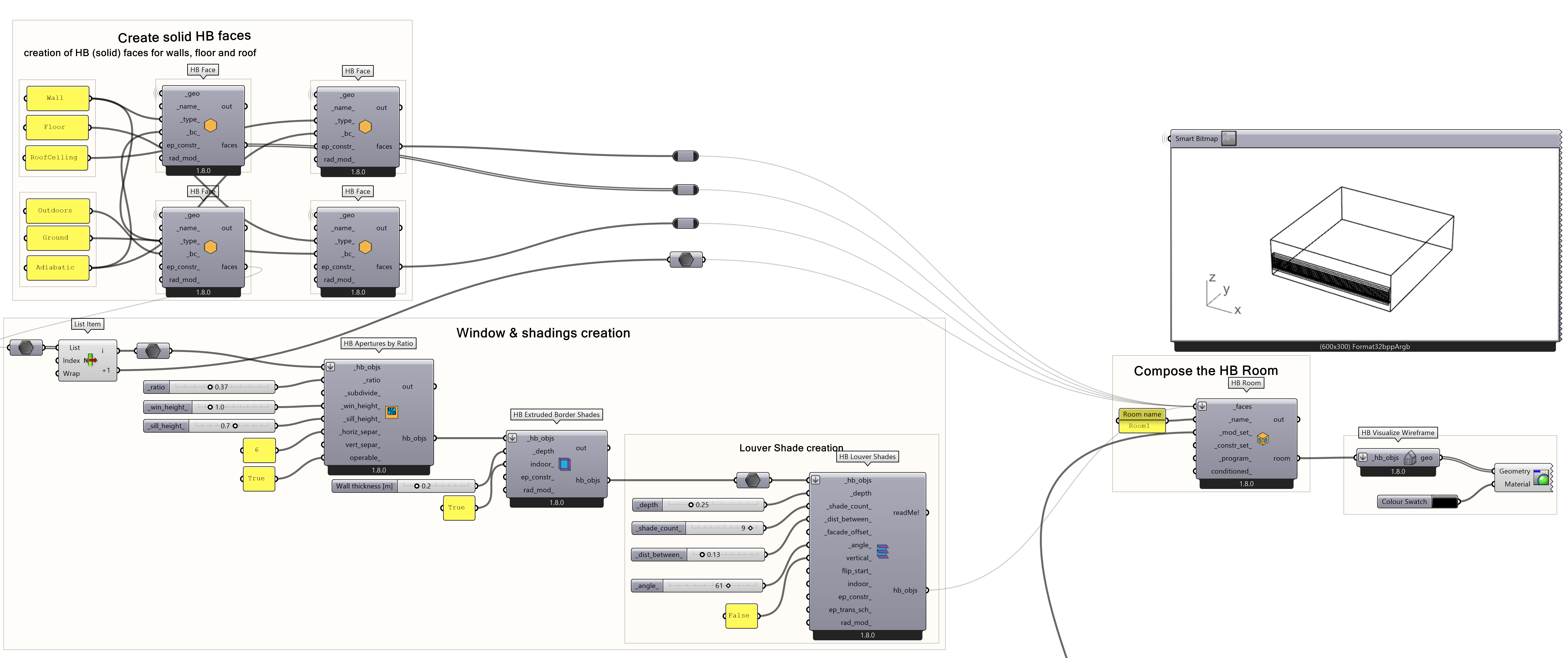
There is a part where necessary HB faces are created. All of them, except for Outdoor Walls, are going directly into the “HB_Room” component later. Now we will focus on Outdoor Walls, as on them we will create the windows.
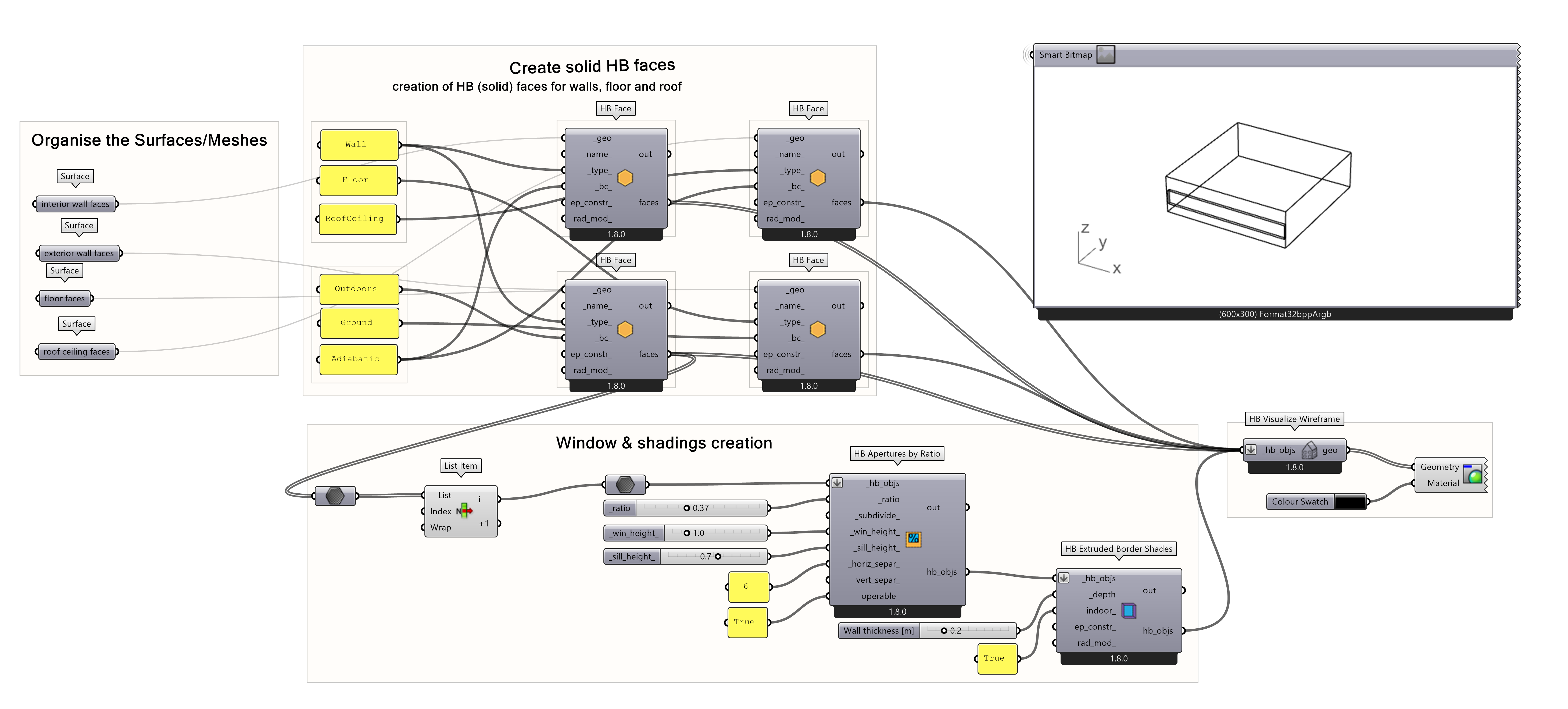
Take the output “faces” of the “HB_Face” “Wall Outdoors” component (bottom left from the set of four on the picture) and connect it to the “list item” component.
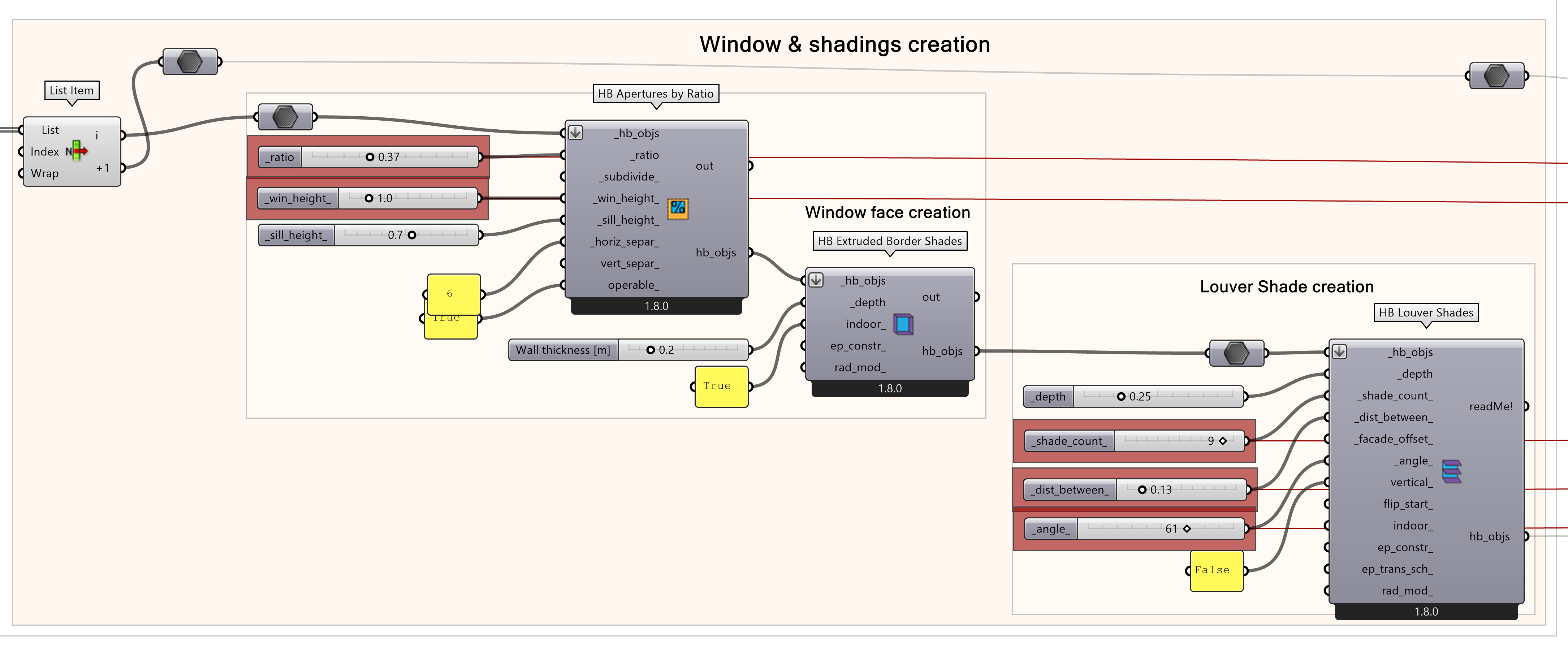
Now, one of those faces is going to be our exterior wall with windows. In case of this example, it happens to be the first output of the “list item” component. To create the windows by ratio, place the “HB apertures by Ratio” component. Connect the chosen face to the “_hb_objs” input. Connect sliders to inputs like so:
- Slider 0.1<0.55<0.9 to “_ratio”
- Slider 0.1<1.5<2.9 to “_win_height_”
- Slider 0.1<0.5<1.2 to “_sill_height_”
- Number “6” to “_horiz_separ_” (ensure two windows)
- Text “True” to “operable_”
This process outputs the wall face with apertures (windows) included. Next, we will add the window rims as shading elements. To do this follow the following steps:
- place the “HB_Extruded_Border_Shades” component.
- connect the “hb_objs” output from the “HB Apertures by Ratio” component to the “_hb_objs” input of the “HB_Extruded_Border_Shades” component.
- Set the “depth” input to 0.2 and the “indoor” input to True.
Refer to the image below for the complete setup.
Louver Creation for HB windows
Now, let’s move on to creating the louver shades for the room. To do this, place the “HB_Louver_Shades” component and connect its inputs as shown below:
- “hb_objs” output of the “HB Extruded Border Shades” to the “hb_objs” input of the “HB Louver Shades”,
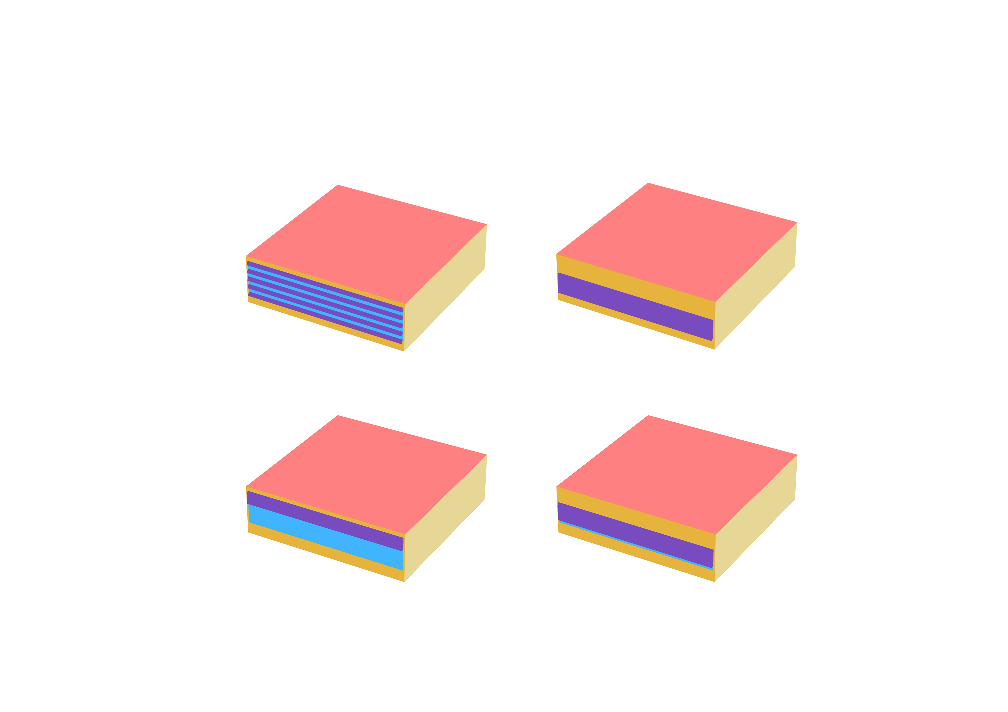
- Slider 0.05<0.25<1.0 to “_depth” input
- Slider 1<5<10 to “_shade_count_” input
- Slider 0.05<0.44<0.9 to “_dist_between_” input
- Slider 0<30<90 to “_angle_ input
- “False” into the “vertical_” input
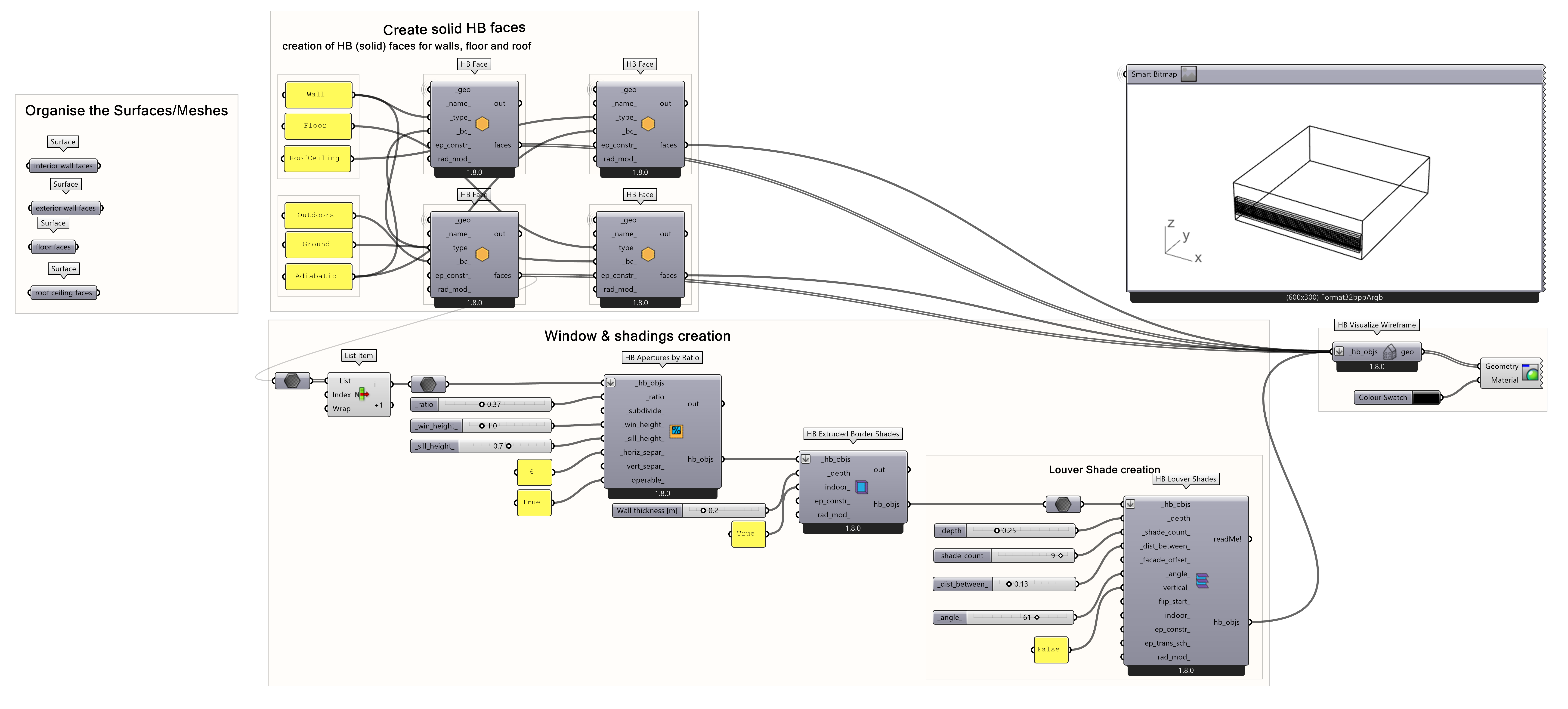
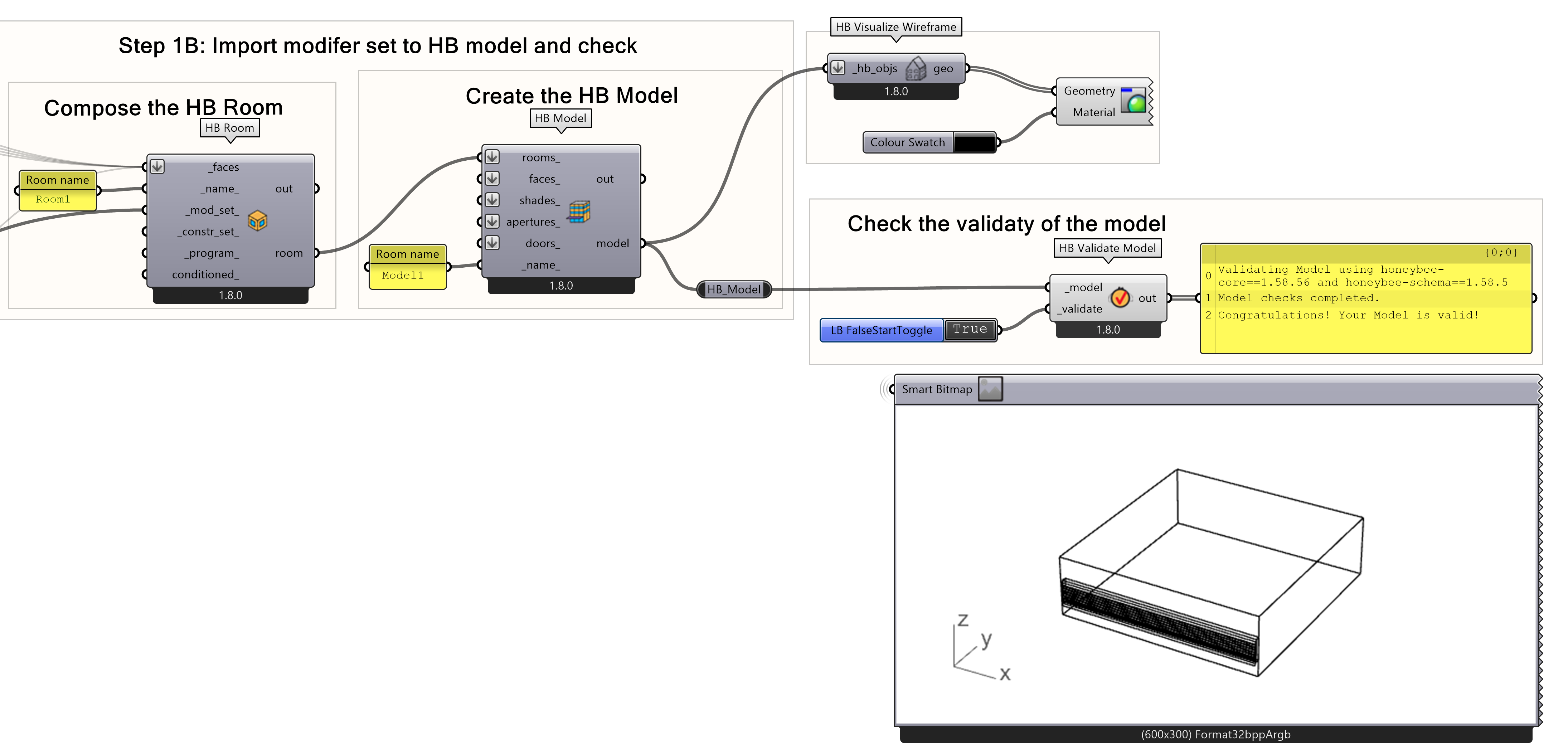
Now, you can connect all the HB faces and objects together into the “_faces” input of the “HB Room” component. See the picture below. If you get an error, it might mean that something is not connected or something is doubled, and all elements do not form a closed room.
Create the HB Model
This part was already explained in the original simulation tutorial, but to quickly recap – here an HB Model is created, and you can check it’s validity with the set of components in the bottom right. Just switch the Toggle to “True”. After you verified the model, you can disable those components, so that they do not run during the Wallacei optimisation process.
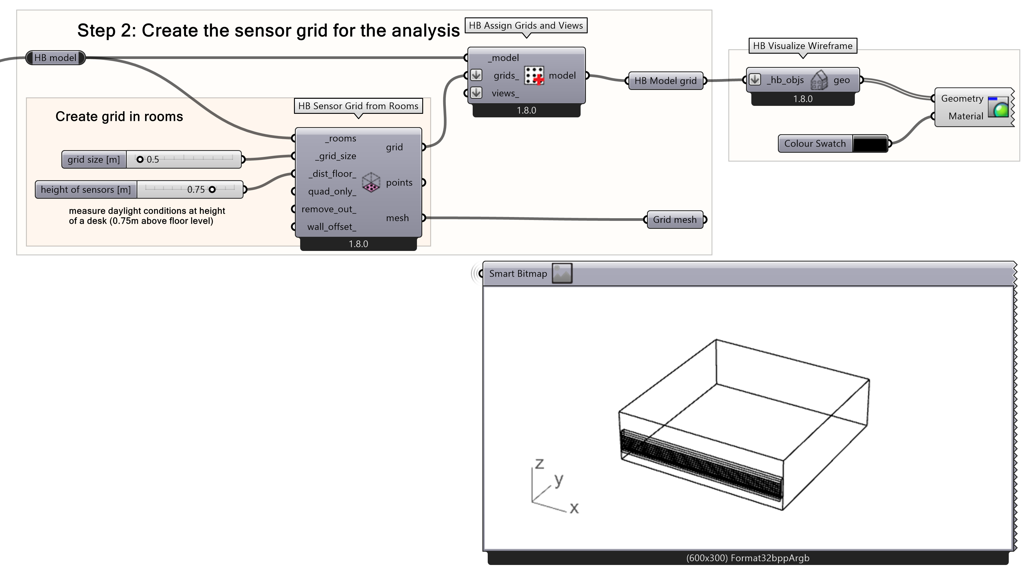
Create the HB Sensor Grid
This part remain unchanged compared to the original daylight simulation tutorial.
Multi-Objective Optimisation – Indoor Daylight 3/6
Simulation Set-Uplink copied
In this example, we want to optimize our window according to the sun hours and annual spatial daylight autonomy. We aim to maximise the number of sun hours during winter, maximise the annual Spatial Daylight Autonomy, and minimise the total number of sun hours during summer. For that we need three separate WEA objects.
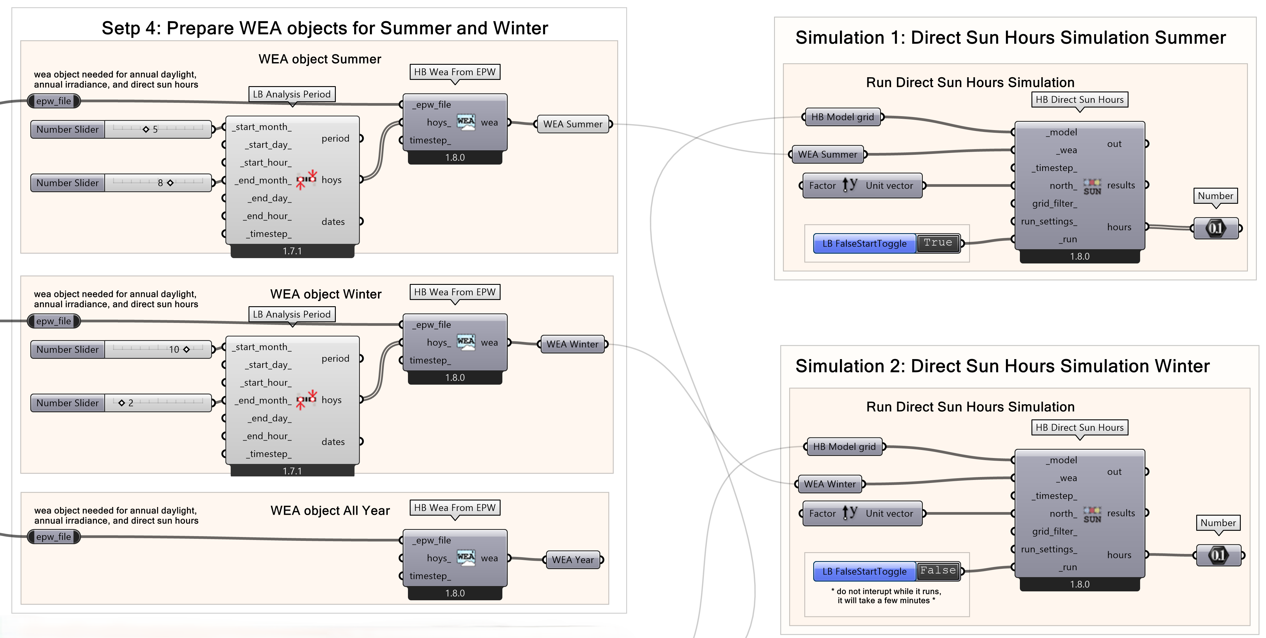
Prepare WEA object for different periods
To create WEA objects, start by obtaining the EPW file and applying an analysis period. Refer to Step 3 on the Grasshopper canvas.
- Place the “HB Wea From EPW” and “LB Analysis Period” components.
- Connect the “epw_file” output to the “epw_file” input of the “HB Wea From EPW” component.
Next, configure the analysis period by:
- Setting the “start_month” and “end_month” inputs of the “LB Analysis Period” component.
- Use 5–8 for summer and 10–2 for winter.
- For an annual WEA object, connect only the EPW file to the corresponding input, leaving the other inputs empty.

Setting up daylight simulations
- Now that you have everything ready, you can now set up the daylight simulations.
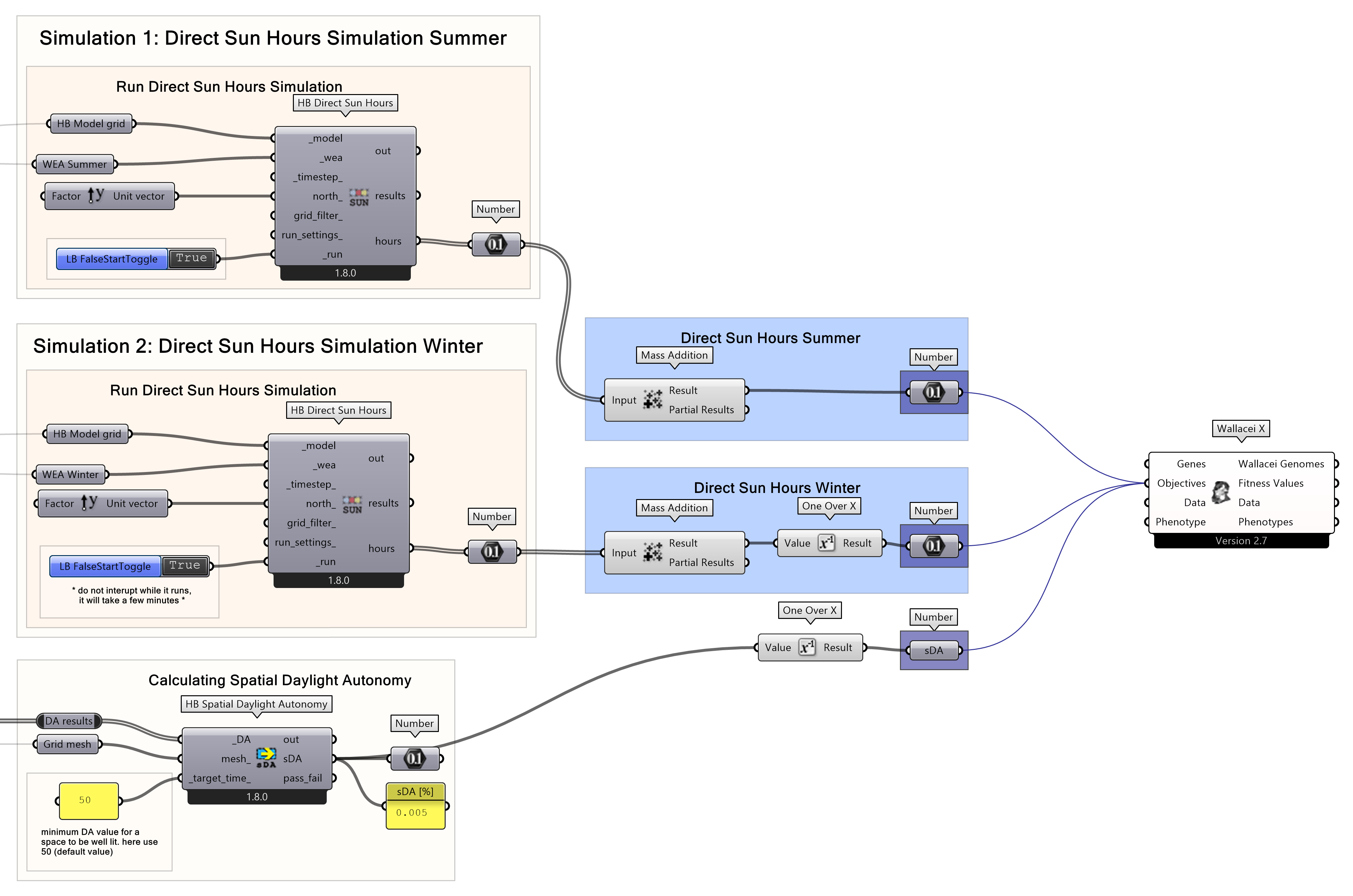
Let’s start with the direct sun hours simulation for summer and winter. - Place the “HB Direct Sun Hours” component.
- Connect the “HB Model Grid” from the “model” output of the “HB Assign Grids and Views” component to the “_model” input of the “Direct Sun Hours” component.
- Connect the “WEA” output of the summer period to the “_wea” input.
- Set the “north_” vector as Unit Y.
- And lastly, connect a Boolean Toggle to the “_run” input, but do not toggle it “True” yet.
Do the same with Winter scenario, duplicating the components, but do not forget to plug the right WEA object.
Next, we must prepare the Spatial Daylight Autonomy simulation, you can do that by followinf these steps:
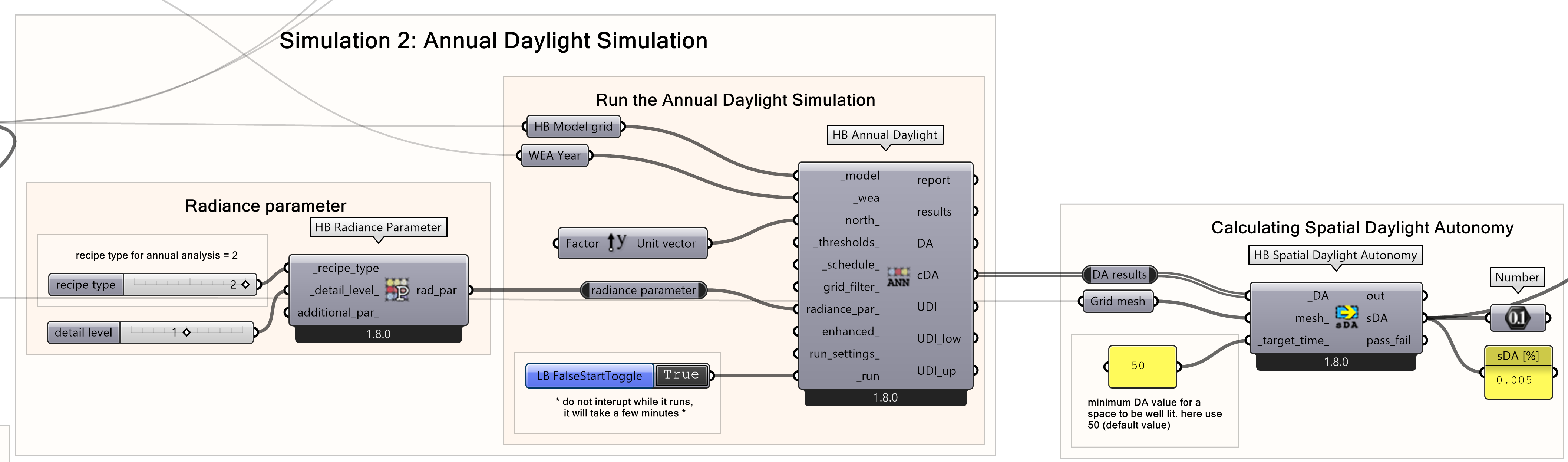
- Place “HB Annual Daylight” component and connect the “HB Model Grid” and the annual WEA object to the first two inputs as per their names suggest.
- Set the “north_” as a Y vector.
- You will then need to set the radiance parameters, set them as in the example file you downloaded at the beginning of this tutorial.
- Connect a Boolean toggle to the “_run” input, do not run it yet.
To calculate the Spatial Daylight Autonomy:
- Connect the results from the “HB Annual Daylight” component to the “HB Spatial Daylight Autonomy” component.
- Attach the “grid mesh” output from the “HB Sensor Grid from Rooms” component to the same “HB Spatial Daylight Autonomy” component.
- Set the Target Time input to 50.
- Use the resulting “sDA” output as the objective for the Wallacei optimization process later.
Multi-Objective Optimisation – Indoor Daylight 4/6
Optimization Set-Up and Runlink copied
In this section of the tutorial, we’ll set up the optimization process for the windows and louvers. This involves defining the objectives, linking the genomes, and connecting the phenotype. We’re assuming you’re already familiar with the Wallacei plugin or have completed the previous Wallacei tutorials. For more information and tutorials on the Wallacei plugin, you can visit the following link:
Objectives preparation
Now it is time to define the objectives for the Wallacei optimisation. In this tutorial we want to minimise the total cumulative sun hours during summer, maximise it for winter, and maximise the sDA annually.
In that case, use the “mass addition” component on winter and summer sun hours simulation results, that way you’ll arrive with just one number for each – the cumulative sun hours number. There is no need to do that for the sDA output as it is already just one number.
As you know, Wallacei is made to minimise objectives, so to have an objective maximised, we must reverse it, using the “One over X” component.
See below a setup of objectives ready to be plugged in to the Wallacei X component.
Preparing the Genome
Go back to the beginning of the script where we defined the HB Apertures and Louver Shades with all the sliders. Here, we are going to find our optimisation variables, or “genes” to connect to the Wallacei X component. You should then connect following sliders to the Wallacei X component:
- Window Wall Ratio – “_ratio”
- Window Height – “_win_height”
- Window Shade Count – “_shade_count_”
- Distance between the shading louvers – “_dist_between_”
- Angle of the louver shadings – “_angle_”
Phenotype
After familiarizing yourself with Wallacei during previous tutorials, you know that we do not have to think about the phenotype just yet. However, we will already prepare the right components for clarity.
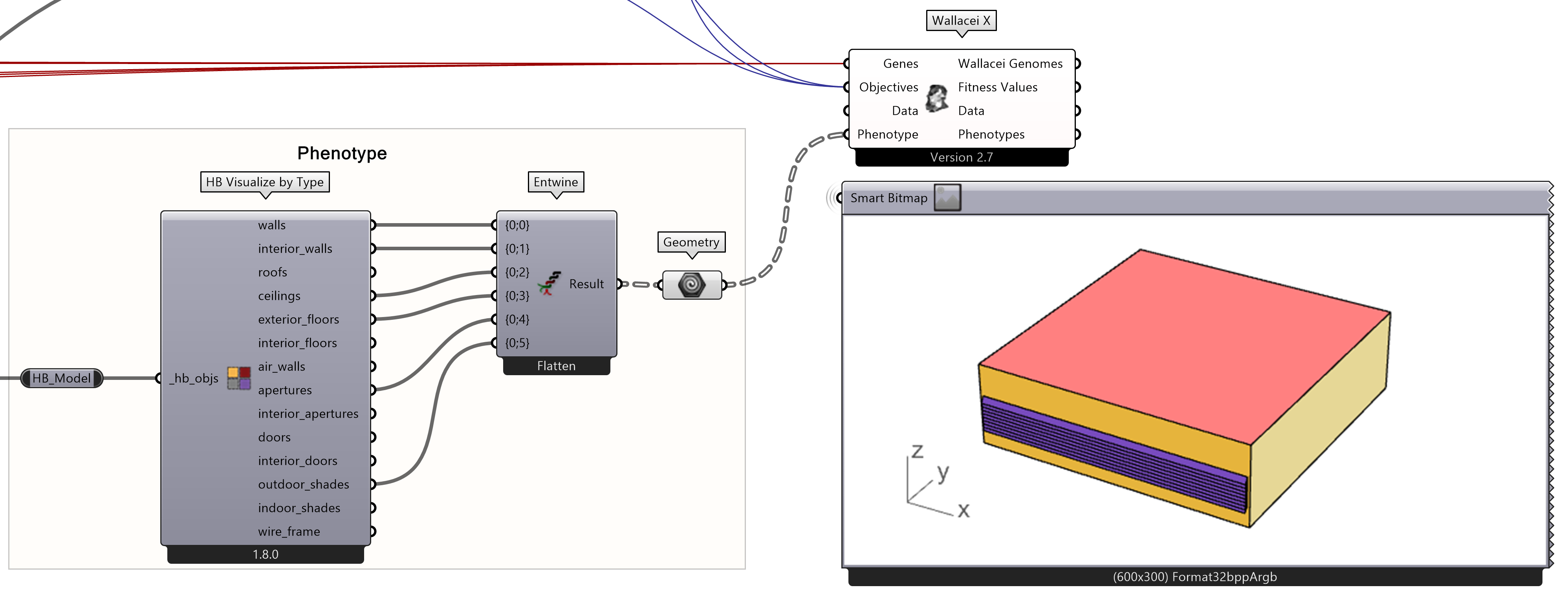
We want to visualize the solutions as HB coloured faces after the simulation. For this we must do the following steps:
- You’ll need the “HB Visualize by Type” component,
- To which you plug in the HB Model, this way you can extract different geometries by their type.
- You can then combine the ones you need through the “Entwine” component. In this example we are going to need: walls, interior walls, ceilings, exterior floors, apertures, outdoor shades.
- You can then plug the “Result” output to the “Phenotype” input of Wallacei X.
Disable all the phenotype related components before running the simulation, as they are not needed yet and would take up computational time.
Wallacei X
It is time for Wallacei to unleash its capabilities. You already know the basics on how to run Wallacei, so we are not going to explain everything here, just the basic options. First, a checklist:
- Disable all unnecessary components that do not contribute to the final objectives
- Toggle all three simulations and make sure they run properly
- Hide all geometry
Open the Wallacei X component by double-clicking on it to access the control UI. Navigate to the “Wallacei Settings” tab and set the “Generation Size” and “Generation Count” to small values, such as 5 or 12.
This is because the Daylight simulations required for this process can be time-consuming, even on high-performance computers. Increasing the number of possible solutions significantly extends the overall optimization time. For a final optimization, you would typically use larger values, but for this tutorial, keeping these numbers low is sufficient to demonstrate functionality and provide useful insights. When you’re ready, click Start.

Analysis and Visualisation
In this tutorial we are not going into detail on how to analyse the Wallacei results. However, let’s see how we can quickly and easily export the results as HB faces to visualise them later. For more details on analysing and visualizing the results, you can check the following tutorials:
In order visualize the results, you must do the following:
- Enable the part of the script where you prepared the HB faces entwined together into one data stream that was inputted into the “Phenotype” of Wallacei X component.
- Then go into the Wallacei X, the “Wallacei Selection” tab and select and export solutions you want, for example, Pareto Front solutions or the last generation.
- After you click export, go back to grasshopper canvas, place the “Decode Phenotype” component and plug the “Phenotypes” output into it.
- Connect the “Meshes List” output to the “Trim Tree” component.
- Then connect the outputted tree to the “Tree” input of the “Tree Branch” component, make sure to simplify the tree.
- Finally, connect a number slider to the “Path” input to visualize each result.
Now you can sort through and visualize the solutions and their geometries.
Multi-Objective Optimisation – Indoor Daylight 5/6
Conclusionlink copied
Congratulations on completing this tutorial!
You’ve now gained the skills to apply evolutionary multi-objective optimization algorithms in Wallacei to tackle environmental challenges like daylight performance using Ladybug and Honeybee simulations. Throughout this tutorial, you explored how to define window and louver creation as variables, set summer, winter, and annual daylight as objectives, and establish your phenotype. Additionally, you successfully set up and executed the optimization process in Wallacei and visualized the results. Take this knowledge further by applying it to your own designs and uncover new possibilities for optimizing environmental performance!
Complete exercise file
Multi-Objective Optimisation – Indoor Daylight 6/6
Useful Linkslink copied
Linked tutorials
Other useful links
Write your feedback.
Write your feedback on "Multi-Objective Optimisation – Indoor Daylight"".
If you're providing a specific feedback to a part of the chapter, mention which part (text, image, or video) that you have specific feedback for."Thank your for your feedback.
Your feedback has been submitted successfully and is now awaiting review. We appreciate your input and will ensure it aligns with our guidelines before it’s published.